决策树 Decision_trees - Ex 3: Plot the decision surface of a decision tree on the iris dataset

决策树/范例三: Plot the decision surface of a decision tree on the iris dataset

http://scikit-learn.org/stable/auto_examples/tree/plot_iris.html

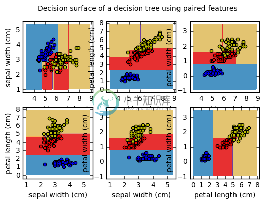
此范例利用决策树分类器将资料集进行分类，找出各类别的分类边界。以鸢尾花资料集当作范例，每次取两个特征做训练，个别绘制不同品种的鸢尾花特征的分布范围。对于每对的鸢尾花特征，决策树学习推断出简单的分类规则，构成决策边界。

范例目的：

1. 资料集：iris 鸢尾花资料集
2. 特征：鸢尾花特征
3. 预测目标：是哪一种鸢尾花
4. 机器学习方法：decision tree 决策树

(一)引入函式库及内建测试资料库

• from sklearn.datasets import load_iris将鸢尾花资料库存入，iris为一个dict型别资料。
  
• 每笔资料中有4个特征，一次取2个特征，共有6种排列方式。
  
• X (特征资料) 以及 y (目标资料)。
  
• DecisionTreeClassifier 建立决策树分类器。
  

import numpy as np
import matplotlib.pyplot as plt
from sklearn.datasets import load_iris
from sklearn.tree import DecisionTreeClassifier
iris = load_iris()
for pairidx, pair in enumerate([[0, 1], [0, 2], [0, 3],
                                [1, 2], [1, 3], [2, 3]]):
    X = iris.data[:, pair]
    y = iris.target

(二)建立Decision Tree分类器

建立模型及分类器训练

• DecisionTreeClassifier():决策树分类器。
  
• fit(特征资料, 目标资料)：利用特征资料及目标资料对分类器进行训练。
  

clf = DecisionTreeClassifier().fit(X, y)

(三)绘制决策边界及训练点

• np.meshgrid：利用特征之最大最小值，建立预测用网格 xx, yy
  
• clf.predict：预估分类结果。
  
• plt.contourf：绘制决策边界。
  
• plt.scatter(X,y)：将X、y以点的方式绘制于平面上，c为数据点的颜色，label为图例。
  

plt.subplot(2, 3, pairidx + 1)
x_min, x_max = X[:, 0].min() - 1, X[:, 0].max() + 1
y_min, y_max = X[:, 1].min() - 1, X[:, 1].max() + 1
xx, yy = np.meshgrid(np.arange(x_min, x_max, plot_step),
                     np.arange(y_min, y_max, plot_step))
Z = clf.predict(np.c_[xx.ravel(), yy.ravel()]) #np.c_ 串接两个list,np.ravel将矩阵变为一维
Z = Z.reshape(xx.shape)
cs = plt.contourf(xx, yy, Z, cmap=plt.cm.Paired)
plt.xlabel(iris.feature_names[pair[0]])
plt.ylabel(iris.feature_names[pair[1]])
plt.axis("tight")
for i, color in zip(range(n_classes), plot_colors):
    idx = np.where(y == i)
    plt.scatter(X[idx, 0], X[idx, 1], c=color, label=iris.target_names[i],
                cmap=plt.cm.Paired)
plt.axis("tight")

(四)完整程式码

print(__doc__)
import numpy as np
import matplotlib.pyplot as plt
from sklearn.datasets import load_iris
from sklearn.tree import DecisionTreeClassifier
# Parameters
n_classes = 3
plot_colors = "bry"
plot_step = 0.02
# Load data
iris = load_iris()
for pairidx, pair in enumerate([[0, 1], [0, 2], [0, 3],
                                [1, 2], [1, 3], [2, 3]]):
    # We only take the two corresponding features
    X = iris.data[:, pair]
    y = iris.target
    # Train
    clf = DecisionTreeClassifier().fit(X, y)
    # Plot the decision boundary
    plt.subplot(2, 3, pairidx + 1)
    x_min, x_max = X[:, 0].min() - 1, X[:, 0].max() + 1
    y_min, y_max = X[:, 1].min() - 1, X[:, 1].max() + 1
    xx, yy = np.meshgrid(np.arange(x_min, x_max, plot_step),
                         np.arange(y_min, y_max, plot_step))
    Z = clf.predict(np.c_[xx.ravel(), yy.ravel()]) #np.c_ 串接两个list,np.ravel将矩阵变为一维
    Z = Z.reshape(xx.shape)
    cs = plt.contourf(xx, yy, Z, cmap=plt.cm.Paired)
    plt.xlabel(iris.feature_names[pair[0]])
    plt.ylabel(iris.feature_names[pair[1]])
    plt.axis("tight")
    # Plot the training points
    for i, color in zip(range(n_classes), plot_colors):
        idx = np.where(y == i)
        plt.scatter(X[idx, 0], X[idx, 1], c=color, label=iris.target_names[i],
                    cmap=plt.cm.Paired)
    plt.axis("tight")
plt.suptitle("Decision surface of a decision tree using paired features")
plt.legend()
plt.show()