决策树 Decision_trees - Ex 2: Multi-output Decision Tree Regression

优质

小牛编辑

132浏览

2023-12-01

决策树/范例二:Multi-output Decision Tree Regression

http://scikit-learn.org/stable/auto_examples/tree/plot_tree_regression_multioutput.html

范例目的

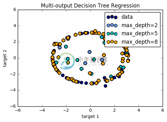
此范例用决策树说明多输出迴归的例子，利用带有杂讯的特征及目标值模拟出近似圆的局部线性迴归。
若决策树深度越深(可由max_depth参数控制)，则决策规则越复杂，模型也会越接近数据，但若数据中含有杂讯，太深的树就有可能产生过拟合的情形。
此范例模拟了不同深度的树，当用带有杂点的数据可能造成的情况。

(一)引入函式库及建立随机数据资料

引入函式资料库

matplotlib.pyplot：用来绘制影像。
sklearn.tree import DecisionTreeRegressor：利用决策树方式建立预测模型。

特征资料

np.random()：随机产生介于0~1之间的乱数
RandomState.rand(d0,d1,..,dn)：给定随机乱数的矩阵形状
np.sort将资料依大小排序。

目标资料

np.sin(X)：以X做为径度，计算出相对的sine值。
ravel()：输出连续的一维矩阵。
y[::5, :] += (0.5 - rng.rand(20, 2))：为目标资料加入杂讯点。

import numpy as np
from sklearn.tree import DecisionTreeRegressor
import matplotlib.pyplot as plt
rng = np.random.RandomState(1)
X = np.sort(200 * rng.rand(100, 1) - 100, axis=0) #在-100~100之间随机建立100个点
y = np.array([np.pi * np.sin(X).ravel(), np.pi * np.cos(X).ravel()]).T #每个X产生两个输出分别为sine及cosine值，并存于y中
y[::5, :] += (0.5 - rng.rand(20, 2)) #每5笔资料加入一个杂讯

(二)建立Decision Tree迴归模型

建立模型

DecisionTreeRegressor(max_depth = 最大深度)：DecisionTreeRegressor建立决策树回归模型。max_depth决定树的深度，若为None则所有节点被展开。此范例会呈现不同max_depth对预测结果的影响。

模型训练

fit(特征资料, 目标资料)：利用特征资料及目标资料对迴归模型进行训练。

预测结果

np.arrange(起始点, 结束点, 间隔)：np.arange(-100.0, 100.0, 0.01)在-100~100之间每0.01取一格，建立预测输入点矩阵。
np.newaxis：增加矩阵维度。
predict(输入矩阵)：对训练完毕的模型测试，输出为预测结果。

# Fit regression model
regr_1 = DecisionTreeRegressor(max_depth=2) #最大深度为2的决策树
regr_2 = DecisionTreeRegressor(max_depth=5) #最大深度为5的决策树
regr_3 = DecisionTreeRegressor(max_depth=8) #最大深度为8的决策树
regr_1.fit(X, y)
regr_2.fit(X, y)
regr_3.fit(X, y)
# Predict
X_test = np.arange(-100.0, 100.0, 0.01)[:, np.newaxis]
y_1 = regr_1.predict(X_test)
y_2 = regr_2.predict(X_test)
y_3 = regr_3.predict(X_test)

(三) 绘出预测结果与实际目标图

plt.scatter(X,y)：将X、y以点的方式绘制于平面上，c为数据点的颜色，s决定点的大小，label为图例。

plt.figure()
s = 50
plt.scatter(y[:, 0], y[:, 1], c="navy", s=s, label="data")
plt.scatter(y_1[:, 0], y_1[:, 1], c="cornflowerblue", s=s, label="max_depth=2")
plt.scatter(y_2[:, 0], y_2[:, 1], c="c", s=s, label="max_depth=5")
plt.scatter(y_3[:, 0], y_3[:, 1], c="orange", s=s, label="max_depth=8")
plt.xlim([-6, 6]) #设定x轴的上下限
plt.ylim([-6, 6]) #设定y轴的上下限
plt.xlabel("target 1") #x轴代表target 1数值
plt.ylabel("target 2") #x轴代表target 2数值
plt.title("Multi-output Decision Tree Regression") #标示图片的标题
plt.legend() #绘出图例
plt.show()

Ex 2: Multi-output Decision Tree Regression - 图1

(四)完整程式码

print(__doc__)
import numpy as np
import matplotlib.pyplot as plt
from sklearn.tree import DecisionTreeRegressor
# Create a random dataset
rng = np.random.RandomState(1)
X = np.sort(200 * rng.rand(100, 1) - 100, axis=0)
y = np.array([np.pi * np.sin(X).ravel(), np.pi * np.cos(X).ravel()]).T
y[::5, :] += (0.5 - rng.rand(20, 2))
# Fit regression model
regr_1 = DecisionTreeRegressor(max_depth=2)
regr_2 = DecisionTreeRegressor(max_depth=5)
regr_3 = DecisionTreeRegressor(max_depth=8)
regr_1.fit(X, y)
regr_2.fit(X, y)
regr_3.fit(X, y)
# Predict
X_test = np.arange(-100.0, 100.0, 0.01)[:, np.newaxis]
y_1 = regr_1.predict(X_test)
y_2 = regr_2.predict(X_test)
y_3 = regr_3.predict(X_test)
# Plot the results
plt.figure()
s = 50
plt.scatter(y[:, 0], y[:, 1], c="navy", s=s, label="data")
plt.scatter(y_1[:, 0], y_1[:, 1], c="cornflowerblue", s=s, label="max_depth=2")
plt.scatter(y_2[:, 0], y_2[:, 1], c="c", s=s, label="max_depth=5")
plt.scatter(y_3[:, 0], y_3[:, 1], c="orange", s=s, label="max_depth=8")
plt.xlim([-6, 6])
plt.ylim([-6, 6])
plt.xlabel("target 1")
plt.ylabel("target 2")
plt.title("Multi-output Decision Tree Regression")
plt.legend()
plt.show()