Lesson 7
Resnet:
We’re going to start by introducing one of the most important developments in recent years: Resnet. Resnet won the Imagenet competition in 2015, and it’s an incredibly simple and intuitive concept. To start, we’re going to use Resnet to perform things we did with Vgg16, such as image classification.
There are different size Resnets, but for our purposes we’re going to use 50 because it works well. In the accompanying notebook, note the argument include_top=False, which simply removes the additional dense layers at the top so we can easily finetune.
Keep in mind that in all of the networks we look at today, we won’t be altering the pre-trained convolutional layers. Therefore all of our training data is simply the output of the convolutional layers. This is fine because in general for images, it’s never useful to retrain the convolutional layers from Imagenet.
Let’s look at what we can do with Resnet.
Finetuning Resnet
First we’ll go ahead and stick a fully connected network onto our Resnet and finetune them for cats and dogs.
In just 48 seconds, this model achieves 98.6 percent validation accuracy, which is incredibly impressive.
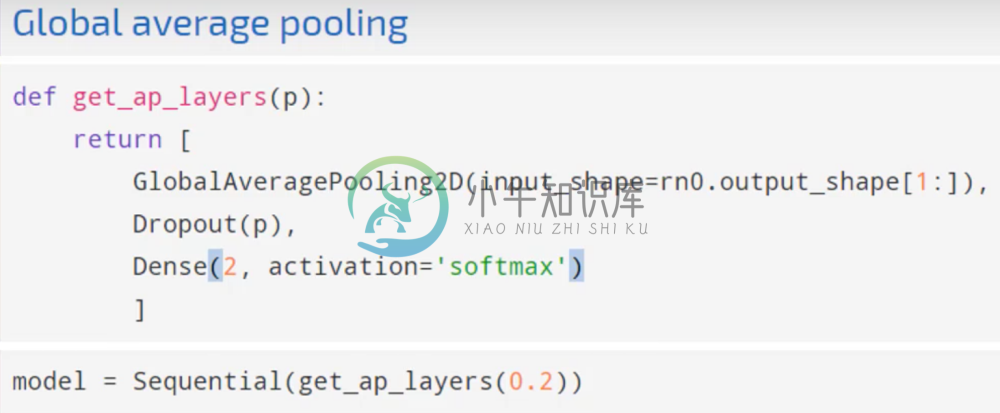
Instead of tacking on a fully connected network, lets use a simple three-layer network that uses something called a global average pooling layer which Resnet is designed to use.
In just 3 seconds of training, this model achieves 98.75 percent validation accuracy.
We could even change the resolution of the image inputs. As an example, let’s change them from 224 by 224 to 400 by 400. After doing this, we get 99.3 percent validation accuracy in about 6 minutes.
Computational Graph=
How exactly does Resnet work?
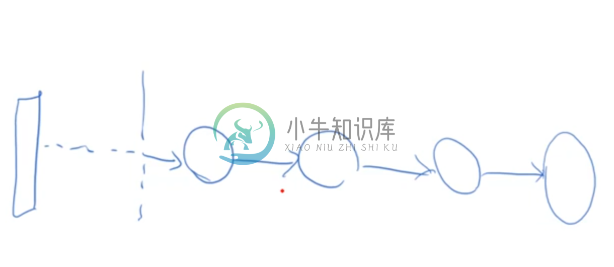
Resnet looks a lot like VGG:
- 3 by 3 Convolution
- An activation layer
- then max-pooling
Each one of these circles is an output of a convolutional layer and a relu activation layer, possibly subject to some max pooling.
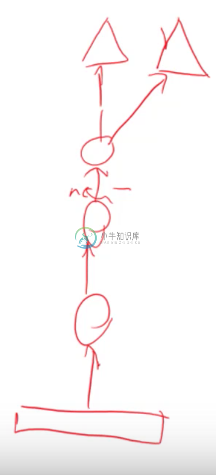
Meanwhile Resnet contains a layer which sums up the previous outputs with the current hidden state.
Where Resnet differs is that after some number of convolutions, the final output is combined with the first convolutional output. However, no transformation is done to the first convolutional layer output; it’s simply added element-wise to the last convolutional output after being acted on by the identity matrix. 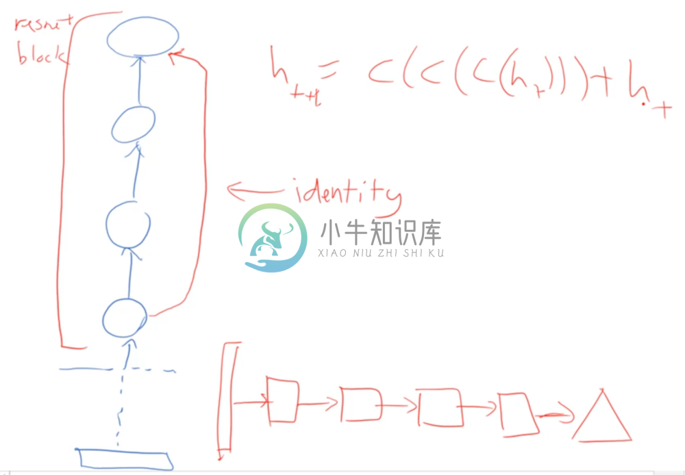
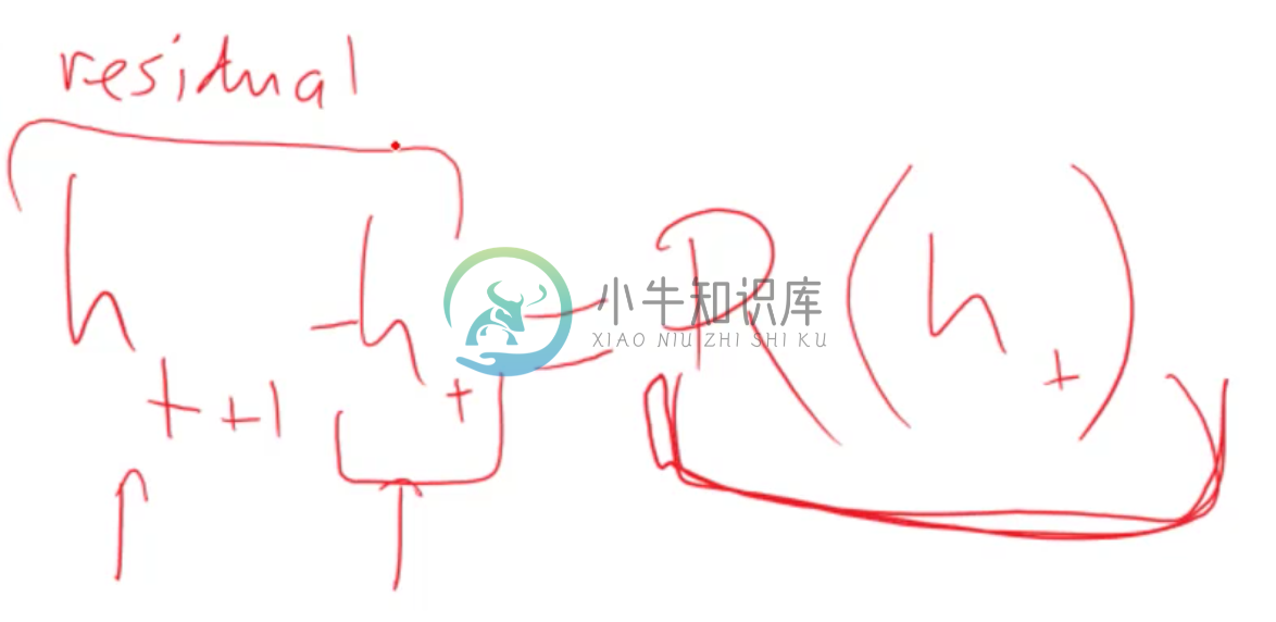
This sequence of convolutions is called a Resnet block, and Resnet stacks a whole bunch of these blocks on top of each other. Consider the hidden state of each Resnet block as indexed sequentially by t. Then the above equation shows that the next consecutive hidden layer outputted by a Resnet block is a composition of convolutions of the previous hidden layer plus the previous hidden layer.
Explaining Resnet
How does this explain how this architecture performs so well?
The author’s intuition was that because back propagation through an identity matrix is easy, Resnet allows for very deep architectures to be constructed with little worry of exploding gradients. This did turn out to be true, as the authors demonstrated with a Resnet of 1000 layers.
However, it’s also been shown that a very wide and shallow resnet with about 50 layers and a lot of activations that did even better. So this first conclusion reached by the authors may not be correct.
Boosting
Their second intuition however still holds. Looking at the equation from before, we can rearrange into:
Where R(h_t) is just the output of the previous hidden layer passing the the Resnet block, which is itself just a composition of convolutions. When written in this format, it’s clear that what the Resnet block is trying to do is to calculate residuals; in other words, the Resnet block is trying to output the difference between the prior layer and the next layer. Then when we add the Resnet output to the prior layer, we hopefully have something that is closer to the desired answer.
This is Resnet architecture is pretty powerful in that by design it automatically learns how to model residuals. This type of architecture works by trying to continuously improve the previously layer’s answers by modeling how that layer differs from the next. You may recognize this as a form of boosting; if you do then you should realize how powerful it is that this change to an otherwise basic CNN architecture is performing boosting on it’s own.
As an aside, it should be obvious that in order to do this operation the dimensionality of the outputs within the Resnet block is the same. Operations like max-pooling are done in between Resnet blocks.
Global Average Pooling
Recall from earlier our simple model that used a Global Average Pooling layer. This layer works similar to max pooling, except that instead of replacing entire areas with the maximum value, it replaces it with the average. In our example, the output of the Resnet blocks is 13x13 with 2048. The way we would implement global average pooling is to take the average of value of all values across the entire 13x13 matrix (hence the term global), and do that for each filter. So the output of global average pooling on the afore mentioned matrix would be 2048x1.
The reason why using global average pooling and one dense layer was more successful than a deeper fully connected network is because Resnet was trained with this layer in it, and therefore the filters it creates were designed to be averaged together. Global average pooling also means we don’t necessarily have to use dropout, because we have a lot less parameters in our dense layers. This of course helps in preventing overfitting, and overall these layers help make models that are very generalizable.
One way to intuit the difference between average and max pooling is in how it treats the downsampled “images” we’re left with after the convolutional layers. In classifying cats vs. dogs, averaging over the image tells us “how doggy or catty is this image overall.” Since a large part of these images are all dogs and cats, this would make sense. If you were using max pooling, you are simply finding “the most doggy or catty” part of the image, which probably isn’t as useful. However, this may be useful in something like the fisheries competition, where the fish occupy only a small part of the picture.
Resnet and Transfer Learning
Resnet is very powerful, but it hasn’t been studied yet for it’s effectiveness in transfer learning. Vgg however is ubiquitous in transfer learning. One reason this may be the case is because the Vgg architecture is designed to create layers of gradually increasing semantic complexity. This lends to easy interpretation and visualization. It also makes it easier for transfer learning, because we’re able to understand what levels of complexity may not be useful for our particular task, and we can intuitively understand what parts of Vgg might need to be finetuned. For this reason, the rest of these architectures are going to deal with Vgg
Data Leakage
Example
In this section, we’re going to be looking at the Fisheries competition from Kaggle. This data consists of photos taken from 12 boats, each boat having a fixed camera that takes daytime and night time shots. Since each camera is fixed, the images from the same boat all have the same general shape and structure. Often times, there are one or more fish in the picture, and the task is to classify the fish.
To start on this competition, we created a simple Vgg model and finetuned it to the fisheries images and classes. We start by pre-computing the convolutional layers, and sticking a few dense layers on top. This simple model gets a validation accuracy of 96.3 percent, which is pretty good.
However there is a problem with our model, and that is data leakage.
Data leakage is the phenomenon wherein something about the target you are trying to predict is encoded in the things that your predicting with, but whatever that something is, it won’t be available in generalizing your data to accomplish the task you want it to do. You can read more about data leakage here.
Source of the Problem
The fishery competition is a good example of this. These different boats fish in different parts of the sea, and they haul in different kinds of fish. Given that each boat has a fixed camera position, the model isn’t actually identifying the fish; rather, it is identifying the boat, and from that inferring what the fish must be.
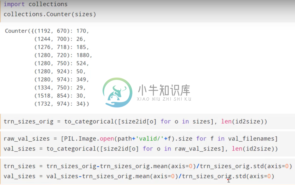
As an example, it turns out that if we use the resolution of the images alone as features for a fully connected neural network, we can achieve a fairly successful model. Why? Because each resolution corresponds to a particular camera on a particular ship. This indicates that what is helping our model predict the fish is not the fish itself, but rather the ship, and this is not a model that will have any success in classifying new pictures of fish. It will just classify based on the ship the image was taken from.
Taking Advantage of Leakage
In developing a useful model for real world application, we would never want to take advantage of data leakage, and would try to do what we can to get rid of it. However, given that this is a Kaggle competition, it’s perfectly fair game to take advantage of it.
In order to do this, we start by making a list of for every file that told us how big that image dimension was for both the validation and training set. These were then normalized by subtracting by the mean and dividing by the standard deviation.
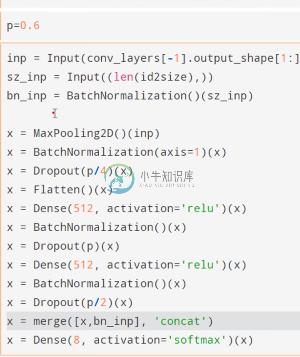
We then rebuild our previous model almost exactly using the functional API.
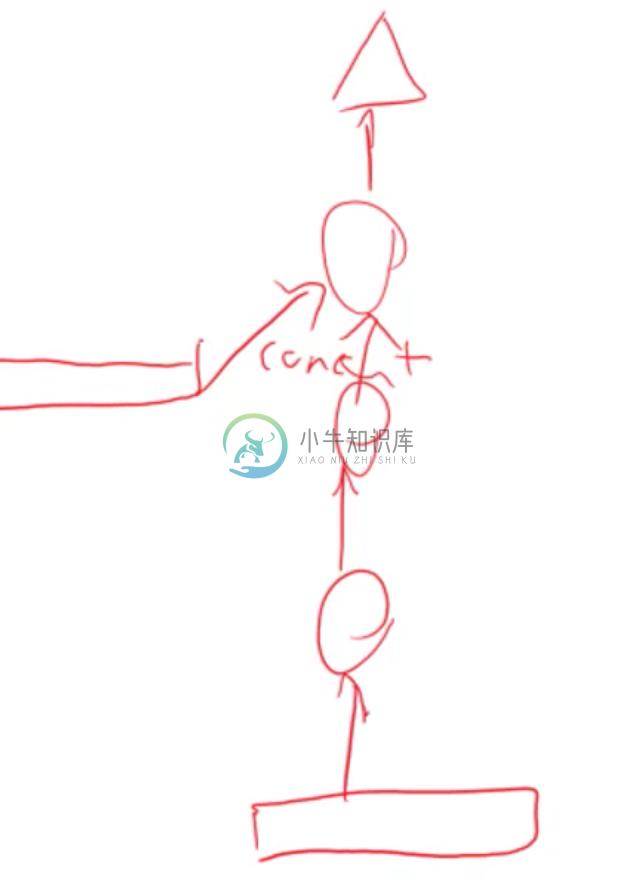
Only now at the every end before calculating a prediction, we concatenate the image size (which has been one-hot encoded and batch normalized) to the output of the penultimate layer in our previous model, and then send this concatenated vector through through one final dense layer for prediction.
We can visualize like this:
Redundant Metadata
Now, that last dense layer learns to combine the image features with the meta data. This is useful in any situation where we might want to use meta data, not just when data leakage is at play. As an example, this could be useful in a collaborative filtering model, where we want to use metadata such as age and gender. In this case, our multi-input model in the fisheries competition out performed our original model at first, but they both ended up fluctuating about 97.5 percent validation accuracy
This is because it turns out that your main data, in this case the image, already encodes the metadata. In this example, while the resolution tells us what boat it comes from, the neural network has already figured out how to tell which boat the picture belongs to from just the image itself. Thus in this case adding the leakage didn’t help our results. Often times it so happens that when people add metadata to models, it ends up being a waste of time because it’s already encoded in the unstructured data.
It’s always important to keep in mind data leakage when working on any machine learning problem. Making sure that your dataset is representative of the actual task you want to solve can help mitigate it.
Bounding Boxes and Multi-Output
In Kaggle competitions, participants can create or find their own data sources as long as they are shared with the community.
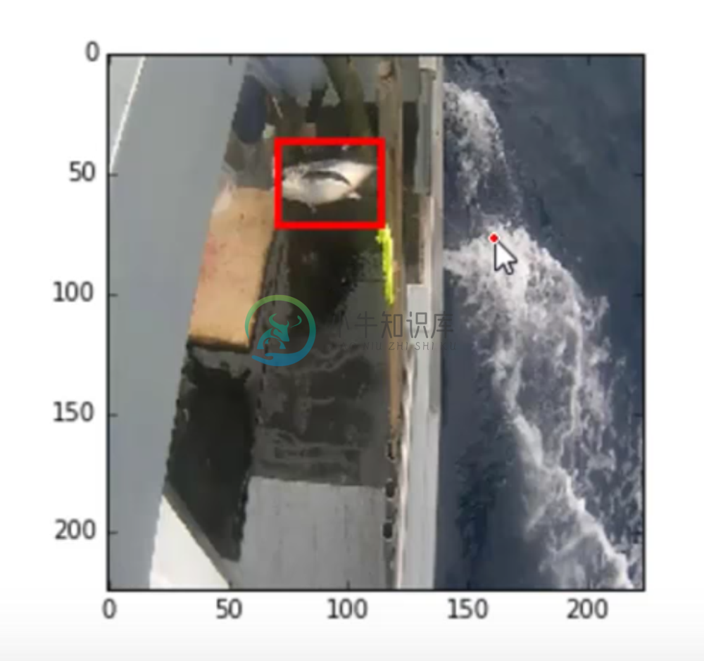
In the fisheries computation, one of the users has went ahead and annotated each image with a box of where the fish is located in the image. This is known as a bounding box. For each image, and for each fish in that image, the dataset gave the height and width of the box as well as it’s coordinates.
From this, we go ahead and grab the largest fish from each image, and create a dataset of with these bounding boxes. For images that didn’t have a fish, the bounding box is simply all zeroes.
Let’s look at an example of one of the bounding boxes.
Building a Multi-Output Model
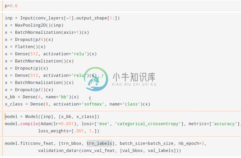
One important problem is that we’re not allowed to augment the test set. In other words, we can’t put bounding boxes on the test set. However, what we can do is use the training set and their bounding boxes to build a model that figures out where to assign a bounding box to a raw image.
Notice that the above model has two outputs; one is simply a linear transformation with no activation, and the other is our normal output. The first output will define our bounding boxes, and the second will perform classification. We use mse as our loss function in the first output and categorical cross-entropy for the second. Training such a model will create dense layers that can do both of those things simultaneously. We also scale the mse loss by 0.001 to make it the same size as the cross-entropy so we allow our network to optimize both evenly. We then use the bounding boxes and fish types as the labels on the training set.
Our model now looks something like this:
With two outputs and one input. Notice that we only have one dense layer for each output. We certainly could have given each output two dense layers, however in this case we want the model to use the same set of features to generate the bounding boxes and the fish classification.
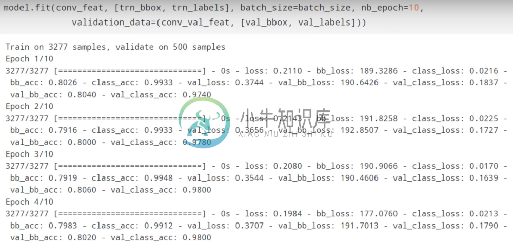
Notice that we now get the loss for each input, as well as the total loss. Here it should make sense why we scaled the MSE; if we hadn’t, it would have completely taken over the loss function, and we want our architecture to optimize well for both tasks.
Relationship between Boxing and Classifying
Strangely enough, this model does better than when we were only trying to classify the fish. The reason behind this is because by forcing the bounding box prediction and the fish classification to share the same features, we’re giving the network a “hint” about what to look for when classifying the fish. Knowing that optimizing for the bounding box will give us some information on where the fish is located, we should intuitively understand that this same information will be helpful in classifying the fish in a localized and general manner. By having our model do multiple outputs, we’ve also made it more stable.
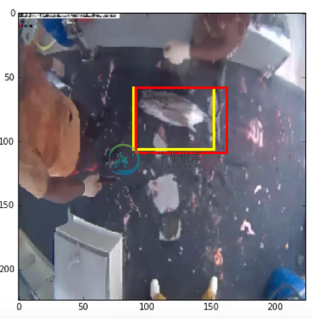
We can take a look and see how well our model predicted the bounding box (yellow predicted, red true).
That’s pretty spot on. It’s astounding that all we had to do to generate these predictions was to just ask the neural net to learn how to do it based off our bounding box labels. Oftentimes before devising some heuristic way to accomplish a task, it’s best to just ask the a neural network to do it and see if it can.
We can extend the efficiency of this model by predicting bounding boxes and then feeding a cropped image of the fish in the bounding box to a classification model. This would most likely result in a very powerful model.
Fully Convolutional Networks
Given a pre-trained model with pre-trained weights, let’s discuss in which situations our model will be sensitive to image size.
With fully connected layers, every input is connected to every output, and therefore it’s impossible to have inputs of different size because it won’t be compatible with the weight matrices.
If the layers are convolutional layers, then we have weights for our filters that slide over the input image. The number of weights here is independent of the image size, but the output shape will depend on the input shape. The Max Pooling layer has no weights, and the batch normalization only cares about the number of weights in the previous layer. So really the only layers that care about the size of the input are the dense layers.
Altering Vgg
Therefore we can alter our Vgg16 class to not only disregard the fully connected layers if include_top=False, but also if we wish to change the input image size to something other than 244x244. This is because if we change the input size, the convolutional layers will still be compatible, but once we flatten their output it will no longer be compatible with the fully connected layers and we can simply build new ones (which we would probably do anyways in finetuning).
Thus if we cut off the architecture before any dense layers, then we can use it on any size input to create convolutional features.
We can try this on something called a fully convolutional network.
In our example, we’re going to set our input size to 640 by 360. It’s important to point out that in images, we specify the dimension in terms of width x height. But when we feed this into the input of our network, it’s going to be row by column, which is the opposite order, so we set our size to be 360 by 640.
We can extend onto the Vgg convolution layers a fully convolutional network.
We can see now that the output shape of our Vgg convolutional layers has changed
This is what we’d expect, given that we’ve changed our input size.
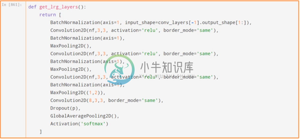
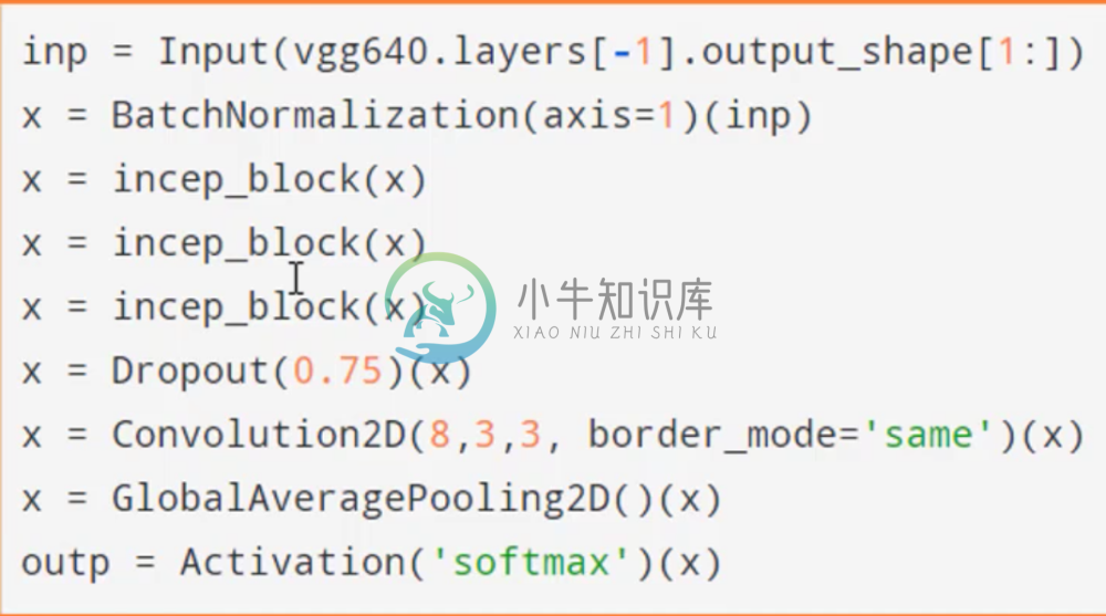
Notice that there are no dense layers in the rest of our network; it’s all convolutions/batch norm/maxpooling, with a final convolution to dropout to global average pooling to softmax.
Several things to note: our final Max pooling is (1,2) due to the rectangular shape of the image. Also, note that our final convolution consists of eight filters. This corresponds to the eight categories of fish, and their are no other weights after this. After this final convolution and dropout, we then do global average pooling across the 8 convolution features, which results in 8 values that we can then use to classify our image.
Heatmaps
This architecture will force the the convolutional filters to find out how fishy each part of the image is, and in particular for what kind of fish. And in training we get a pretty stable result of 97.6 percent validation accuracy in 30 seconds. In fact on the Kaggle set, this architecture landed in the top 30 results.
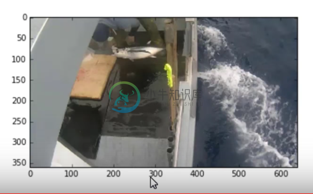
One cool thing about this architecture is that it preserves a sense of the original image right up to the moment of classification. We can use the output of the last convolutional layer to see what the activations look like (refer to the notebook to see exactly how this is done). Given this input:
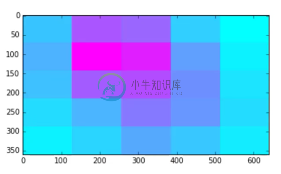
we get the following output:
And so we can see that it’s figured out where the fish is in the picture.
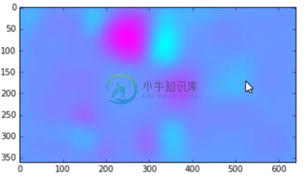
We can modify this network to produce heat maps that will show us what our convolutional layer is activating on, which is a remarkable visualization technique. To modify, we simply remove the max-pooling layers, which maintains the 22x40 dimension of them image. It doesn’t give as accurate results, but we have a higher resolution to visualize the heat map. We can resize the heat map back to 360 by 640 through interpolation.
Now, for the same input as above, we get:
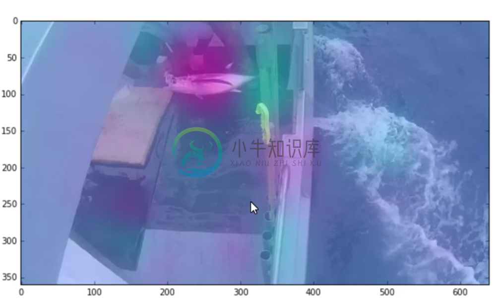
Which is much more detailed. We can now stick one on top of the other
And this tells us a lot. We can see that this particular filter of the eight, which activates on albacore, is doing a good job at activating over the fishy part of the image and not really anywhere else.
In fact, if we looked at the filter for “no fish”, these colors would be reversed as we might expect. The areas that are pink that are not fish are suggesting that the model is looking at things like parts of the boat. This could indicate that there is still some data leakage present.
Inception CNN
Another successful architecture is the Inception CNN. A combination of Inception and Resnet won this year’s Imagenet competition.
Below is a very small implementation of an Inception net:
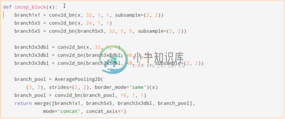
Where are inception blocks are defined as:
We can see that basically what it’s doing is concatenating the output of multiple different convolutional filter sizes. Each Inception block allows us to look for features at different scales at each stage. before passing to a fully convolutional network.
Our results with this network are good, but not on par with some of our earlier architectures. The real takeaway here is to just familiarize yourself with these sorts of architectures, as they will be much more prevalent in the second part of this course.
Like Resnet, Inception hasn’t been well studied in regards to transfer learning.
Accompanied with the above architectures introduced, previous techniques that have been applied to the VGG16 model can be done here as well, such pseudo-labeling and data augmentation.
Reviewing RNNs:
Most of the focus of this course has been focused on CNN’s because it is ubiquitous amongst most use cases. Having said that, there are many challenging problems that are being solved with RNN’s such as speech recognition and language translation. They are also useful in cases of e-commerce transaction, logistics, and in general time-series problems.
Last week, we built an RNN nearly from scratch in Theano. We say nearly because we allowed Theano to calculate the gradient. In this review we are going to look at how the gradient is calculated. This is not a task to be done every time by hand, however for educational purposes and better understanding of back propagation we are going to try it out this one time.
RNNs In Python:
In order to show how to do this, we’re going to write an RNN completely from scratch in Python. The reason why we’re choosing to do this for an RNN is because it’s really one of the more difficult cases of back propagation.
Transformations, Activations, and Derivatives
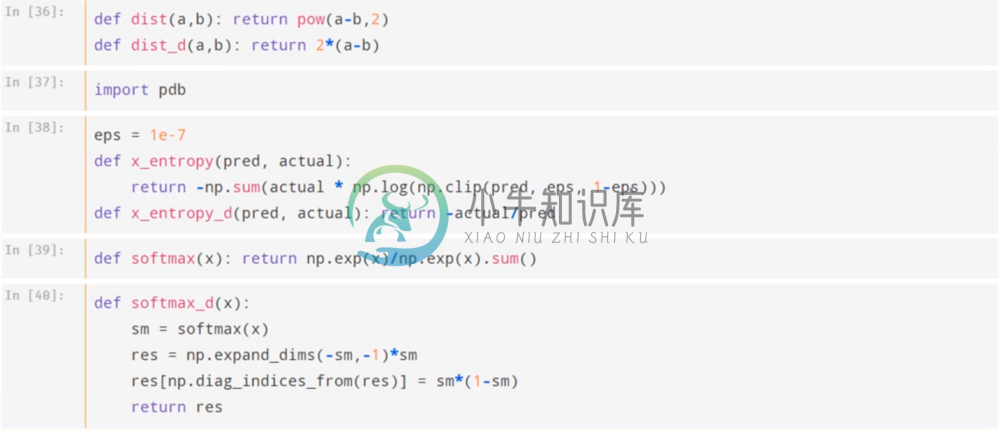
Here are the essential functions to calculate the sigmoid and relu activations. For each one, we also provide a function to calculate their gradient. We’ve also done the same for the euclidean distance
Below we do the same thing for our cross-entropy function, as well as the softmax activation.
When writing these functions, you should always double check that the answers you get with your versions match Theano’s.
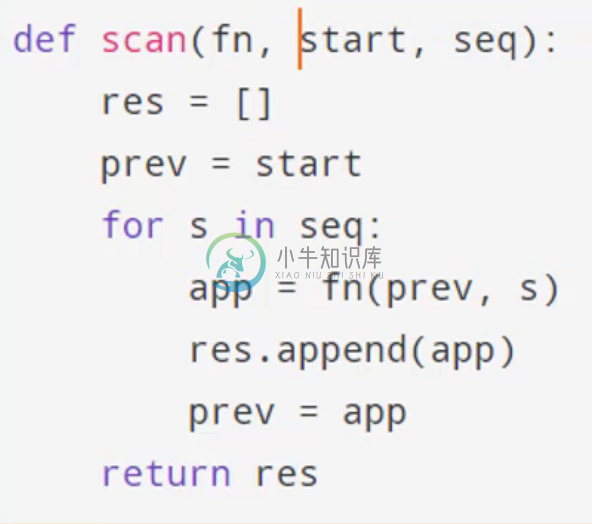
Scan Function
Then finally, we write our scan, which you should recall from last lesson. While we don’t actually need a scan in python, Theano uses a scan because the GPU parallelizes it’s processes instead of iterating through a for loop, so we include the scan function for consistency.
As a reminder: the scan function allows us to go through a sequence one step at a time, where we apply a function to each element of that sequence. At each time step, we pass as parameters to the function the next element of the sequence, and the result of the previous call. In order to do this we also provide an initial value.
Forward/Backward Pass
We’re going to train our RNN on the Nietzsche corpus with one-hot encoding for words.
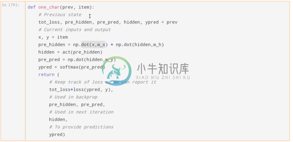
First we are going to do a forward pass by going through each character and applying the function appropriately. Below we define the forward pass function to get the hidden state. This is similar, but less optimized than theano’s function.
To get the hidden state, we apply the input weight matrix to x, the hidden weight matrix to the previous hidden state, add them element-wise and pass through our activation. We then make a prediction using the new hidden state with the output weight matrix and pass through the softmax activation.
Note that our function keeps track of the total loss by adding to the previous loss our new loss for these predictions and labels. In addition we also keep track of the weight matrices to use in back propagation, the new hidden state for the next forward pass, and our predictions.
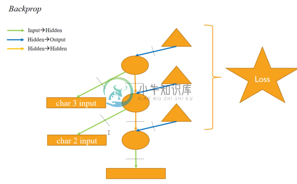
Now we’re ready for the backward pass. We can use the following image to visualize it.
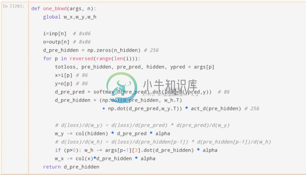
We can follow the backwards pointing arrows to calculate the derivatives of each parameter using the chain rule. Recall that the loss function is the sum of the losses for each of the outputs.
In a backward pass, we create a partial derivative of the output in respond to the input. This tells us at what rate changing the input could effect the output. To follow up and do this process through out the whole network, we use the Chain Rule. The idea is to essentially “undo” all the transformations and activation functions.
The above code works backwards through the respective transformations to calculate each partial derivative via the chain rule, updating the weights as we do so via gradient descent with our learning rate. Take some time to really work through this and understand what’s going on.
Training
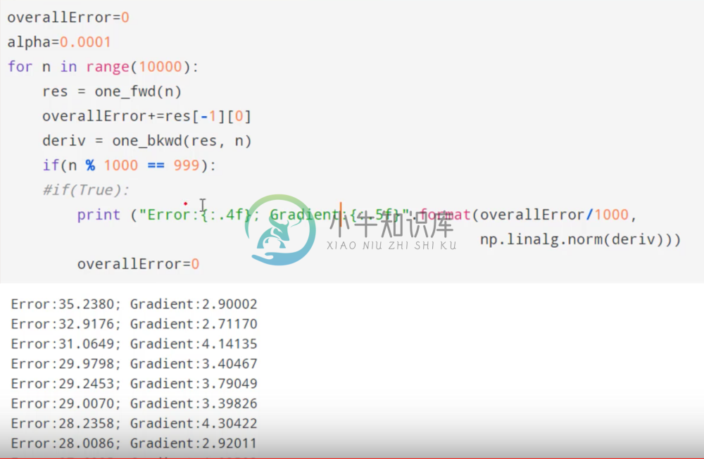
Now that we’ve defined our forward and backward steps, we initialize our weights as normal, and then we can loop through our data set and train our network.
We can see that our network is starting to minimize our loss function.
For more details, refer to Lesson 7 Notebook.
Advanced RNN’s: the GRU
Let’s look at two advanced versions of vanilla RNN’s.
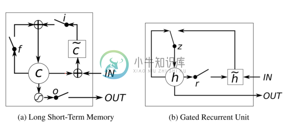
LSTM’s have been quite popular, but today we’re going to focus on the GRU because they are simpler and better. Both architectures are meant to prevent gradient explosions using the gates that each sequences goes through.
A GRU operates almost like a normal RNN. The input and weight components work exactly the same. However, there is something more complicated happening in the self loop on the hidden layer. When we look on the left side of the loop, it appears to come back to itself but it runs into a gate. So this isn’t just a normal loop.
Let’s look at what happens on the right hand side. We can see that the hidden state is going to go through another gate. A gate is simply a mini neural network that outputs a bunch of numbers between 0 and 1 which we multiply with the input to the gate. The “r” at this gate stands for reset; if the numbers were all 0, then what would come out of that gate is nothing but zeros. This would allow the network to “forget” the hidden state, and so when combining with the new input, we actually are just getting the new input with no previous state. On the other hand it could be al 1’s, which would allow the network to completely remember the hidden state.
How do we figure out if we want to remember or forget? We don’t know, which is why we implement this gate with a little neural network that takes as input the current hidden state and the new input. Thus it will learn a set of weights that will tell it when to forget what it learned from the previous state.
Whatever comes through the gate, we will call h tilda. This is the new value of the hidden state after being reset and combined with the new input. Now, this h tilda and the original hidden state are combined in the update gate. If the value of the gate is 1, then the update comes purely from the previous hidden state; if it’s 0, it comes purely from h tilda. Otherwise it is a mix of both. This is determined again by another neural network.
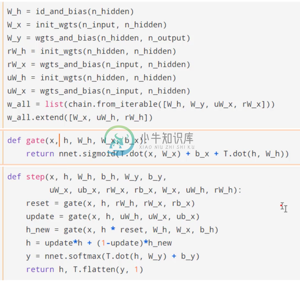
We can see below how to implement this in Theano.
We’ve initialized the weights for the respective gates, and implemented the gates into our our hidden loop as we’ve described. What’s cool about this network is not only is it simple, but it has the ability to learn these special sets of weights that know to throw away state when it’s a good idea. These extra degrees of freedom allow SGD to find better answers.
Lesson resources
- Lesson video
- Forum discussion
- Lesson 7 notes
The notebooks:
The python scripts:
- VGG with batch normalization - also adds ‘size’ and ‘include_top’ parameters
- resnet50.py - The resnet architecture
