Lesson 6
This week’s links
- The lesson video and timeline
The notebooks:
Information about this week’s topics
- Introduction to Theano
- Theano convolution tutorial
- Designing great data products - Jeremy’s paper on how to use predictive modelling to optimize for actions
- A Simple Way to Initialize Recurrent Networks of Rectified Linear Units - Geoffrey Hinton et al.
Assignments
- Practice building your own models in Theano to develop your understanding of the library prior to next week’s class
- Study up on the chain rule if you’re feeling rusty (e.g. on Khan Academy)
Pseudo Labeling: MixIterator
Recall from Lesson 4 the Pseudo Labeling technique LINK for semi-supervised learning. As a reminder, pseudo labeling is a way for us to learn more about the structure of data when we have a large amount of unlabeled data available to us in conjunction with labeled data. The basic premise is to train a model on the labeled data, and then predict labels in our test set. We can then go back and build another model using the training set and the pseudo labelled test set. This is applicable in instances where we have a very large unlabelled test set in comparison to our training set, such as in the Statefarm competition.
Of course, the goal is to use the pseudo labelled data to add to the knowledge gained when training on the labelled data, and therefore it’s important to control how much of the data in each batch is pseudo labelled. Typically, we’d like to only have 1⁄3 to 1⁄4 of the batch come from the pseudo labelled data.
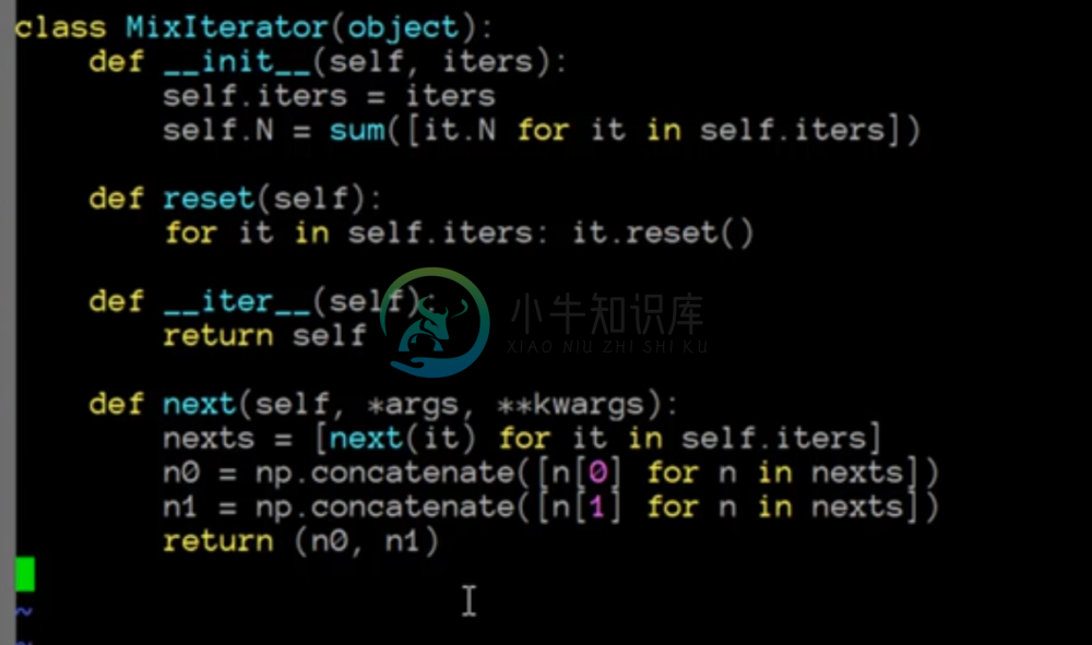
Keras doesn’t have a way to create a batch generator that allows us to pull from different sources, so Jeremy has put together a useful code snippet that does just that.
Embeddings Revisited
Before we move on to new topics, we’d like to take a moment to review embeddings.
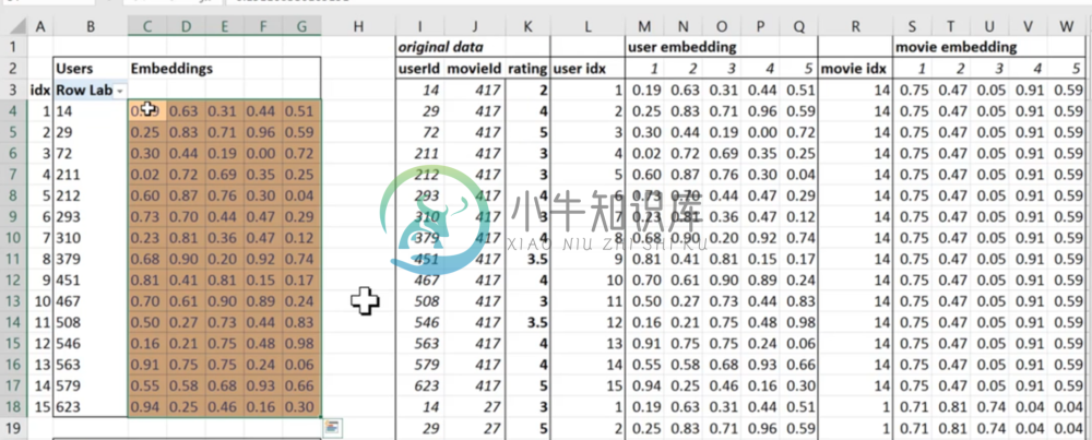
When we originally looked at embeddings in Excel, we represented them in a cross-tabular format bordering a matrix that represented the rating of each user for each movie. We then trained a model by calculating our response for each user/movie pair as the dot product of their embeddings, plus a bias term for each, and we used gradient descent to optimize these parameters.
This is a useful representation do demonstrate the idea of embeddings, but is completely impractical in reality to store these scores as a matrix. We would expect the matrix to be extremely sparse, given that there are typically only so many user-movie combinations, so it’s wasteful to store the ratings in this format.
Embeddings in Keras
Below we can see in excel how Keras represents embeddings, and what our inputs are.
The raw data, listed under “original data” is what our inputs are. The embeddings are stored in embedding matrices; to the left we can see the embedding matrix for users. When keras receives this input, it’s passed to the embedding functions for both the users and movies, and looks up the index where that user/movie id is. We now have two embeddings for the user/movie id, and these are taken as the numerical input to our model (be it a simple dot product or a neural network). Then the third element of the raw data is simply the target, in this case the rating, and we use this to calculate our loss function and update the embedding matrix, according to gradient descent.
As we mentioned last lesson, this is identical to creating one-hot encodings for every user and movie id, and then multiplying by their respective matrics. The embedding lookup function simply uses less resources.
Text Embedding Example
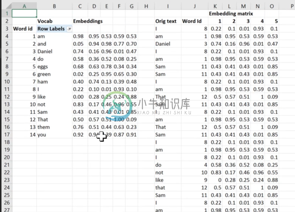
Our previous example using ratings as a function of the embeddings was simple enough. Let’s see how embeddings can represent words in text, in this case from Suess’s seminal work “Green Eggs and Ham”.
On the right, we have a sequence of words that make up the poem, each with an id specific to the word and an embedding. On the left, we have the embedding matrix for each unique word, initialized to random values and each index corresponding to the word id. We’d like to emphasize again that the numerical value of the id’s are meaningless; they just tell us where to find the embeddings in the embedding matrix.
Recurrent Neural Network (RNN):
[](http://wiki.fast.ai/index.php/File:Lect_5_rnn.png “Enlarge”)
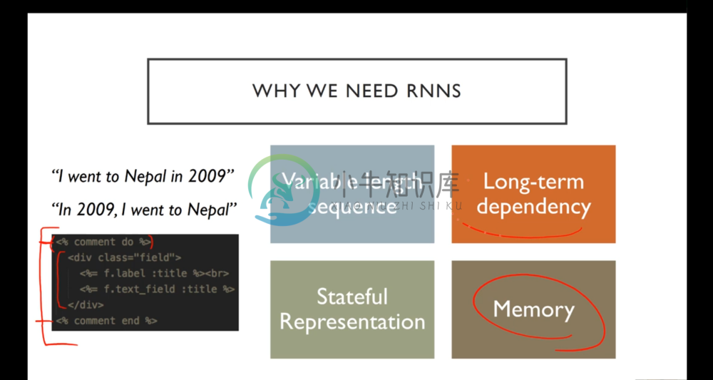
Let’s continue to dive into Recurrent Neural Networks. Recall from our introduction last lesson that RNN’s are all about memory; we’d like an architecture that can keep track of things that have happened in the past to inform what should happen in the future. For example, in structure data like text we would like a model to know to close a quote after opening one, and in order to do so it needs to remember that the quote was opened in the first place.
Computational Graph Review
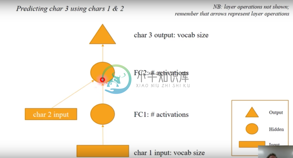
Let’s go over our computational graph representation from last lesson.
Each colored box represents an matrix of activations. Specifically:
- Input matrix (Rectangular shaped)
- Hidden activation matrix (Circular shaped)
- Output matrix (Triangle, output shaped)
Arrows show “layer operations”. We perform an operation from one color box to make another colored box. These operations consist of:
- A linear function or convolution
- An Activation function, such as Relu or Softmax.
Two arrows going into the same shape means that the shape is the result of adding the outputs of those two layer operations
- Typically this will represent summing up the layer operation outputs element-wise
The above example represents a network that takes as input an embedding for a char, applies two layer transformations to it, then combines with a transformed input of the next character. This combination then finally goes the a final layer operation to provide a prediction for the third character.
Recall that the reason why we add in the second character later is to give the network a sense of state. In other words, we don’t feed in character 1 and 2 to a model independently, rather the final matrix before the output is something that is built off the the second word, and the first word, so it necessarily encodes information about that first word.
Time-Shift Invariance
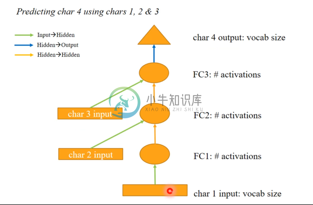
Next let’s look at an example architecture for predicting the fourth character.
Observe that there are essentially only 3 kinds of layer operations at work here.
- Those layer operations that turn a character input into a hidden layer (green arrows)
- Those layer operations that turn one hidden layer activations into new hidden layer activations (orange arrows)
- Those layer operations that turn hidden activations to output (blue)
We can note that the green arrows are all weight matrices of the same dimensionality. In fact, we can see that the orange arrows are all the same dimensionality as well.
The similarity doesn’t stop there. Consider that every green arrow is performing the same task, which is to find the best way to take a character and convert it into a hidden state. The orange arrow is trying to find the best way to take hidden state from a previous character and combine it with hidden state for the next character. And the blue arrow is trying to predict a word, given a hidden state. We might reasonably assume that these tasks are completely independent from whether or not we’re looking at character 1 and 2 or character 32 and 33. In other words, these tasks should be independent of shifts in time, meaning the task for transforming and combining words 1 and 2 are the same for words 5 and 6. Note that when we say time, we’re referring to sequential behavior.
Predicting Nietzche w/ a Fourth-Letter Model: The ‘3 Char Model` section of the lesson6.ipynb notebook
Let’s actually build the previous model in Keras and use it to predict Nietzche, by training it on a corpus of his work.
Pre-Processing
Here is how the above Neural Net can be built in Keras:
- We use Nietzche’s work as input text.
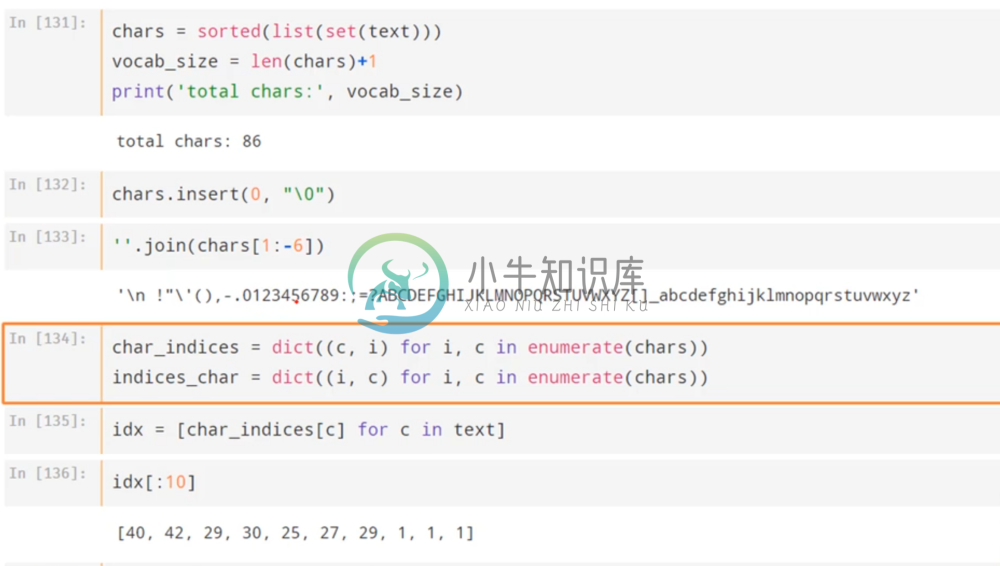
- We find the unique characters in the text corpus (alphabetic letter with symbols). Note that vocab_size is +1, because we are adding a NULL value to use as a placeholder later, so don’t worry about that right now.
- Then we create a mapping for the characters to ids, similar to the words from the poem earlier. Now we can represent the text as a sequence of numeric values.
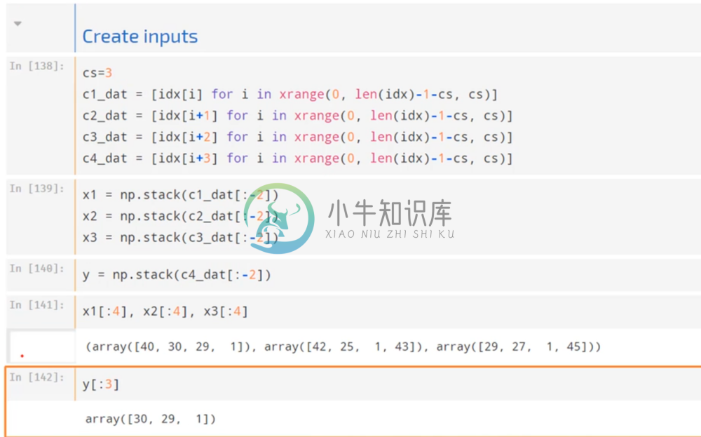
Our task now is to predict the fourth character, given a sequence of three. The first step is to go through our corpus and for each (non-overlapping) sequence of four characters, denote which ones are the first, second, third, and fourth and stack them into separate numpy arrays. Our individual inputs are now the first, second, and third characters, and our target is the fourth.
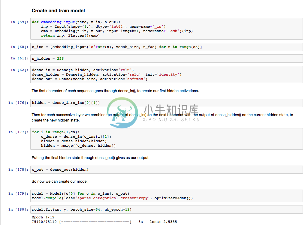
Next, we create an embedding matrix for each character, which we will pass our ids to. Note that this is actually unusual for this sort of task. Oftentimes a one hot encoding is used, but we believe that an embedding will help capture more nuanced information about each character in regards to the objective.
Model Construction
Now we can pass our embeddings to a dense layer. In our example, we settle on 256 activations.
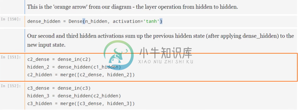
Remember that we want to use this same dense matrix for different inputs. So far in defining the layer, we have yet to attach it to any input. So what we’ve defined so far is simply the weight matrix.
Now when we define the hidden layer for character 1, we can simply use that weight matrix and apply it to the character 1 embedding. We can use the same weight matrix again for our other characters, and this layer represents our green arrows.
In the same spirit, we will define another dense layer to represent the orange arrows for going from hidden layer to hidden layer. Again, on defining this layer we won’t attach to anything; instead we’ll apply this same weight matrix to different inputs.
Now we can build the merging portions of our network using these two layers
And finally we’ll create our blue arrows, which transforms the hidden state into a prediction. We can then build our model.
Prediction Results
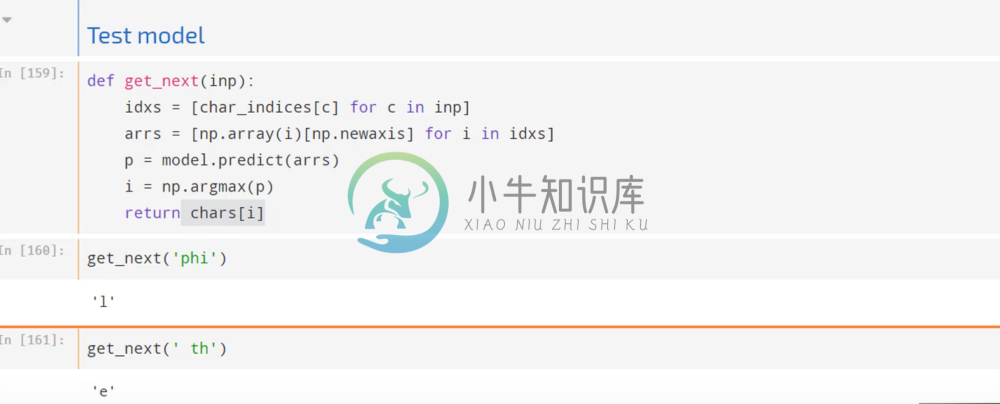
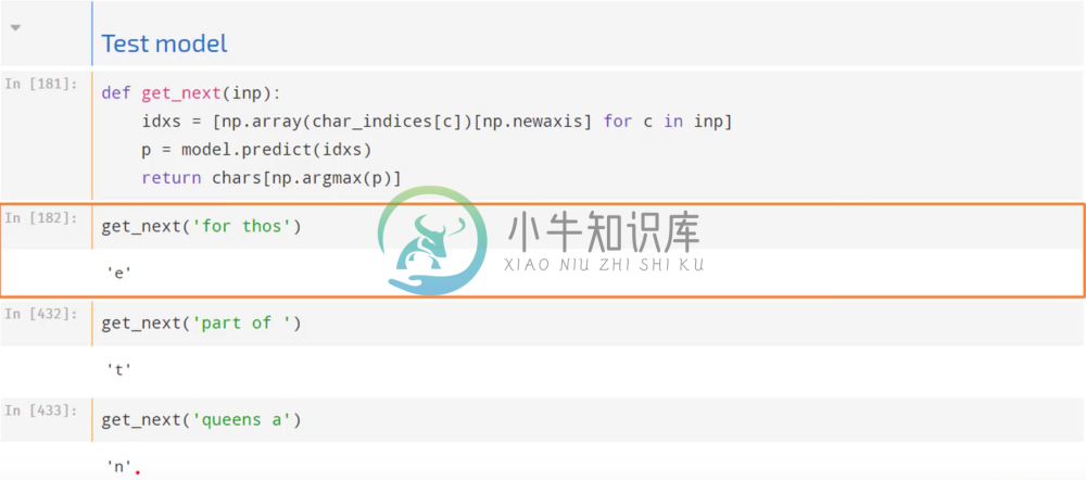
After training over many epochs, we can test it on sequences of three characters.
We can see it knows how to finish “phil” and “ the”, so that’s nice. But it’s not particularly powerful just yet, because it does not take into account any context other than the previous three characters.
However, what is powerful is that we’ve demonstrated how easy the Keras functional API makes it to construct arbitrary architectures.
N-th Word Model
Recurrence
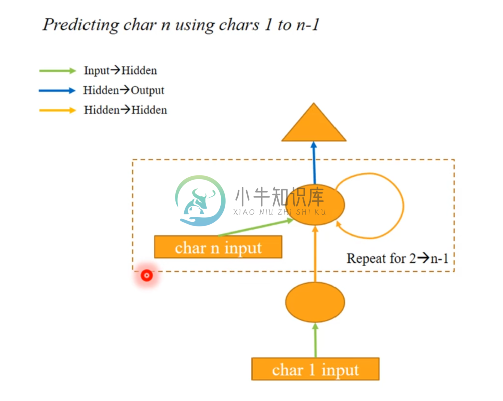
Next, let’s move on to the more arbitrary task of predicting the n-th character given a sequence of the previous n-1 characters. As with the previous approach, it will be a recurring process, by which we mean the same matrices will be applied on each new input and new hidden layer. This recurring behavior is what defines an RNN, and to emphasize this behavior (and to compactly represent it) we can simply stack all the input/hidden layers on top of each other into this new computational graph:
This is what we called the RNN’s recurrent form. Our previous representation was what we call it’s unrolled form. It’s important to note than when stacking Keras on Tensorflow, it can only implement RNN’s in the unrolled form. Theano can actually implement the RNN in it’s recurrent form, which is more efficient.
Pre-processing
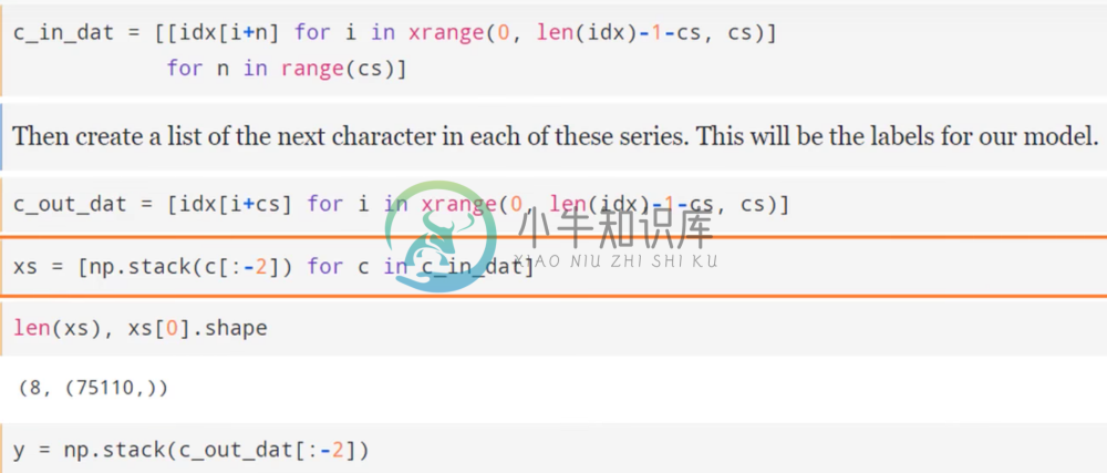
Now lets look at how to easily implement an RNN for predicting the n-th character (where cs is n-1).
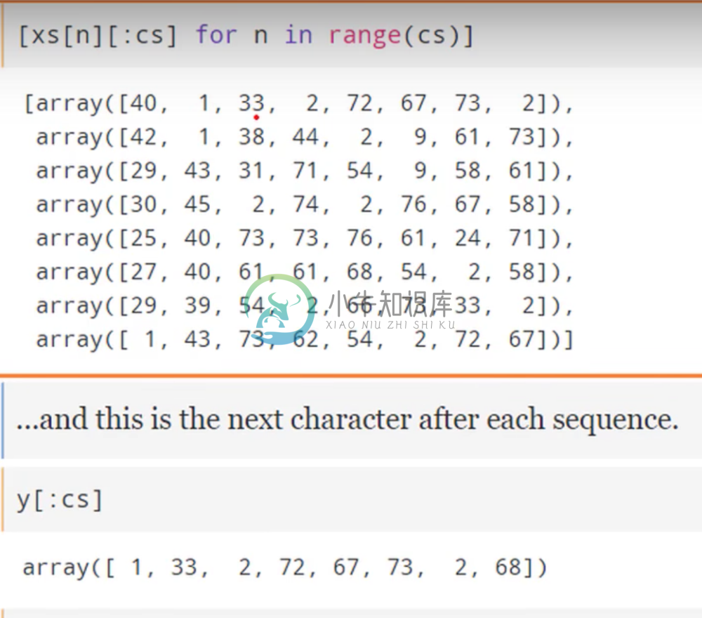
In this example, we’re trying to predict the ninth character, so we can construct our input matrix and target with the following (where cs=8):
And we can visualize them below:
We can see in our input matrix, sequences of 8 word id’s that represent eight consecutive words. In our y matrix, we have the id of the next word corresponding to each input sequence.
Model Construction and Results
Now we can create and train the model.
We would expect this model to achieve better results than our previous one, given that it keeps track of more state. Indeed, in our example we get a loss of 1.8 compared to 2 in the previous model.
We can see this in action as before:
These all seem reasonable.
This type of RNN that predicts one output given a list is best suited for a task such as sentiment analysis. For example, if our input was a tweet, an appropriate use case would be to use the entire sequence of a tweet to predict the sentiment.
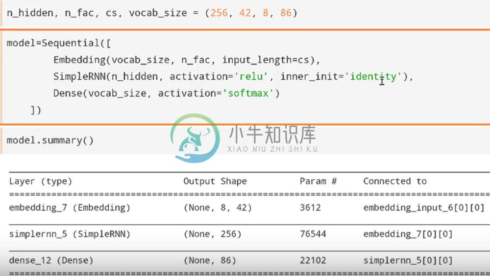
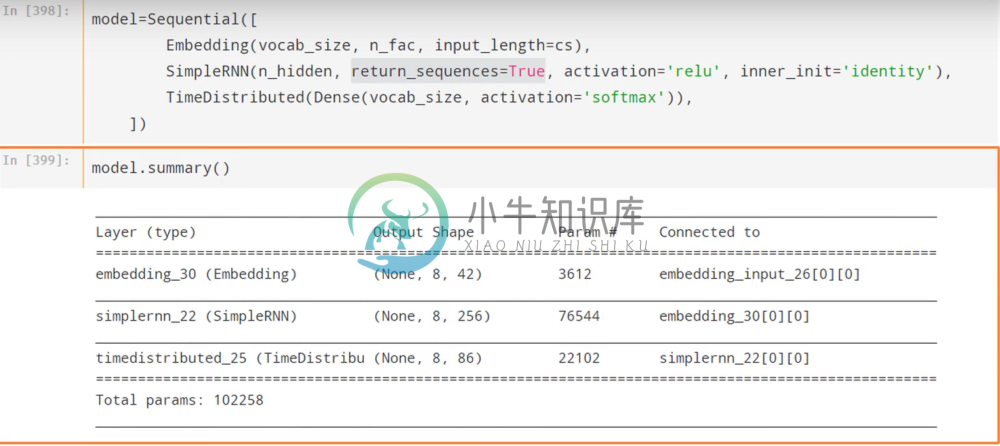
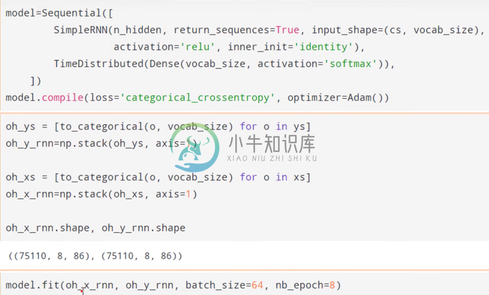
This type of RNN is very common, and fortunately Keras supports a built in implementation of it that we can compile into a simple sequential model as shown below.
Hidden Layer Initialization & the Identity Matrix
One thing to note is that we’ve atypically initialized our hidden-to-hidden weight matrices to be the identity matrix. In the context of keeping track of state, this makes sense. Recall that the hidden-to-hidden layer transformation is telling us the best way to transform the information from the prior state before combining it with the new transformed input. It’s reasonable to assume that a good place to start in this transformation is to do nothing; in other words, let’s start by passing the exact information from the prior state into the construction of our new state, and let SGD inform us as to the optimal way to to do this.
Further, empirical evidence suggests that in initializing the hidden-to-hidden layer weight matrix as the identity and the activation as ReLu, we can achieve very powerful results.
Sequential RNN
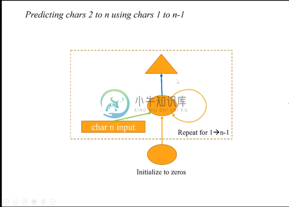
Let’s now consider the following RNN architecture:
Sequential Output
Note that unlike our previous RNN’s, we’ve included the output matrix (represented by the triangle) in our iteration box (dash line box). What this means is that we’re now allowing our model to predict a sequence of characters. Specifically, given a sequence of characters 1 to n-1, we’re going to predict characters 2 to n by generating an output at each iteration.
This is a good idea because it increases the amount of predictions we can make on our training set, which increases the amount of updates we can make through back propagation. If we only output one prediction for every sequence of n-1 characters, then we only have as many predictions as there are sequences in the corpus. Now, we have n-1 times that many predictions, and we can learn alot more. This also helps in building an RNN that can truly handle long-term dependencies or context. Typically in any similar sequence-to-sequence task, we want to construct a similar architecture.
In altering our previous model, the output now looks like this:
This is simply the input sequence shifted over one character. Now, the first character will predict the second, the first and second will predict the third, and so on and so forth.
Model Compilation & Fitting
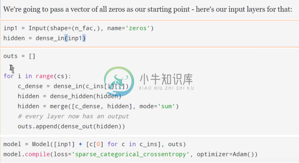
Notice in our new graph that our input is now a vector of zeros. This is because we’d like to move our first character into the recurrent process, but we still need some vector to initialize the first hidden layer and so we just use a vector of zeros.
Now we define the three layers as before, and we can construct this new model giving a sequence of outputs like so:
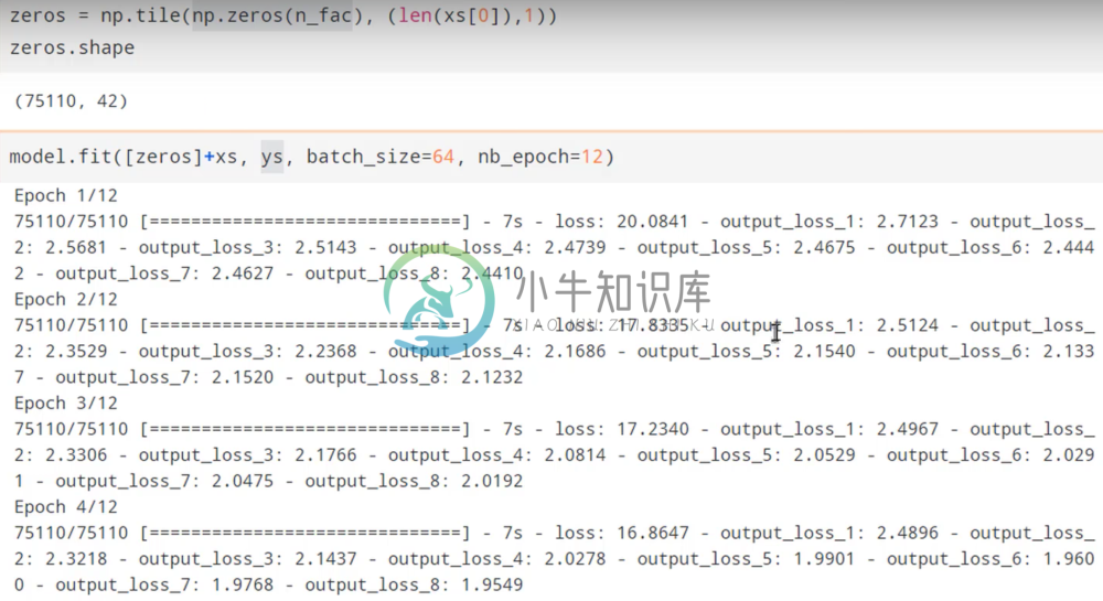
Next we create our zero vectors, and add them to the inputs upon training.
Note that the output of our training gives us losses for each individual character we’re predicting, i.e. the first, second, third, etc. Note that the more characters we have to predict with, the better our loss. This makes sense given that we have much more context to predict the eighth character than we do the third.
Model Results
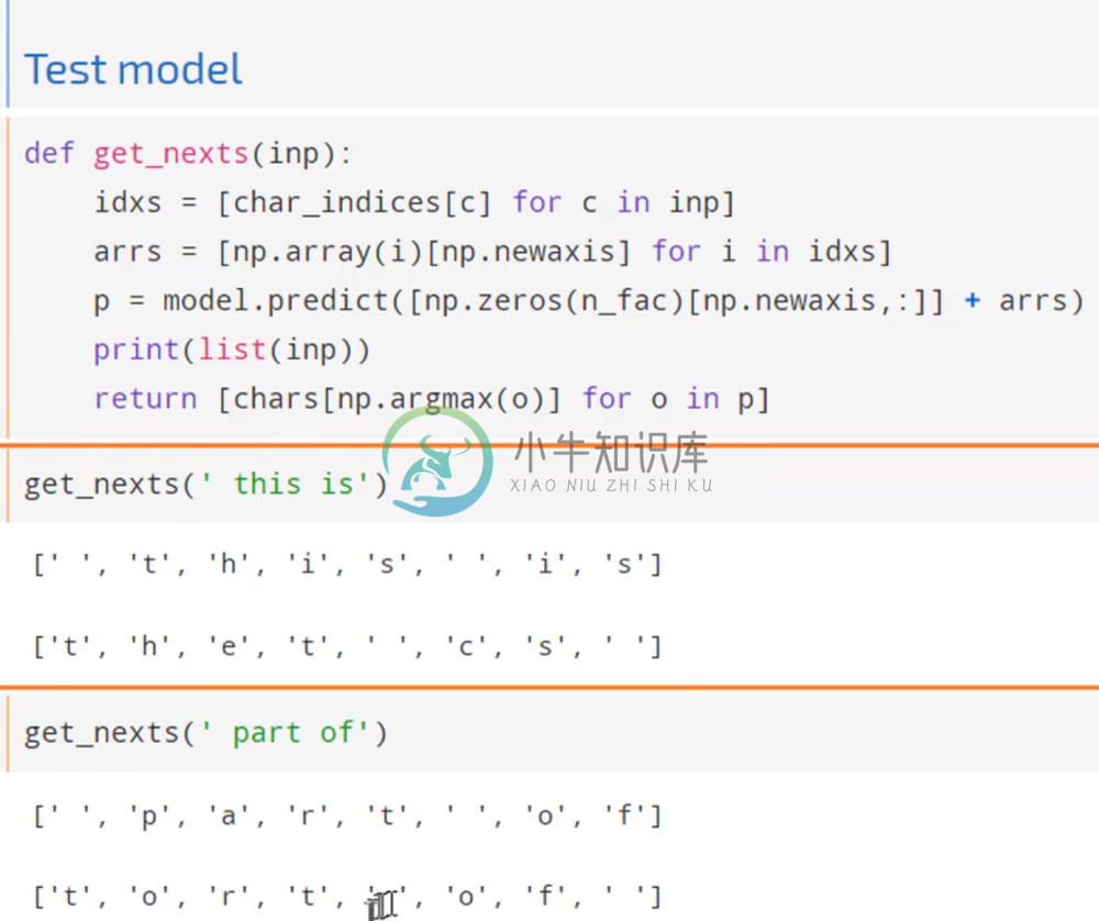
We can again test this sequence model out:
Each index of second vectors show the predictions of that word, given the inputs of the first vector up to that index. So for example, we can see that after the model reads in “ this”, it predicts that the next character should be a space. It also knows that after a space, we should start a word. In the second example, we can even see that after reading in “ part “, it was able to successfully predict that the next word was “of”.
This model is able to use sequences of eight to create context like before, but it’s learned a lot more by predicting in this sequential way.
Sequential Model in Sequential API
In Keras, it’s very easy to create this model in the Sequential API.
As we can see, it’s almost identical to our previous model, only we’ve included setting the parameter return_sequences=True which moves the prediction step into the iteration. The only other difference now is that we also have to change our targets into the necessary sequences.
Stateful RNN
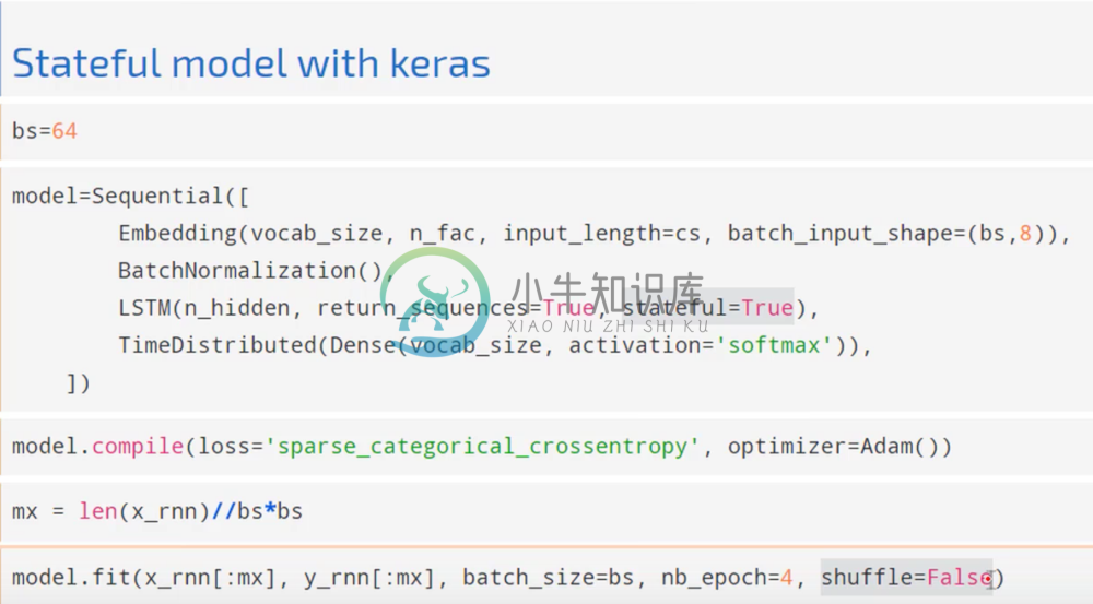
These models are cool but for our purposes we’d really like to create more state, meaning we want models that can handle long-term dependencies. In order to do this, we can’t train on random batches of our data as we have been doing, so we have to make sure to set shuffle=False.
Secondly, in order to keep track of long term dependencies, we need to pass along our hidden states from sequence to sequence. In other words, while we will have an original input of zeros, we need to pass the final hidden state on that sequence of 8 to the next sequence of 8, thereby keeping a hidden state that represents an arbitrarily long dependency.
Stateful RNN in Keras
In Keras, constructing these stateful models is simple:
All we had to do here was to add stateful=True to our model to tell it to pass the hidden layers from sequence to sequence. We also made sure to keep our ordering by setting shuffle=False.
Training Stateful RNN’s
Training these stateful models is a lot harder than our previous models. This is because unlike in our previous model where our hidden-to-hidden layer operation was only applied to the hidden layers eight times, it’s now being applied to it possibly hundreds of thousands of times. This makes it sensitive to exploding gradients; if the matrix is even slightly scaled poorly, a number that’s slightly larger than the others will be raised to a very large exponential and will destabilize the network by sending the activations to infinity.
This instability was so problematic that these models were thought to be untrainable until the creation of the Long-Short Term Memory (LSTM) model. We’ll discuss this model in more detail next week, but the idea is to actual replace the orange hidden-to-hidden looped with a neural network that decides how much of the state matrix to keep/use at each activation. By having this neural network which controls how much state to use, it learns how to avoid gradient explosions and create an effective sequence.
As an example of the difficulty in training these networks, a simple RNN layer wasn’t able to produce results. In fact, replacing it with an LSTM layer had no luck either, and we were only able to see success after inputting a batch normalization layer before the LSTM.
One thing to note is that these stateful models will run slower because it has to do each sequence in order, which makes it more difficult to parallelize. Over time however it will produce much better results.
Stateful RNN Example
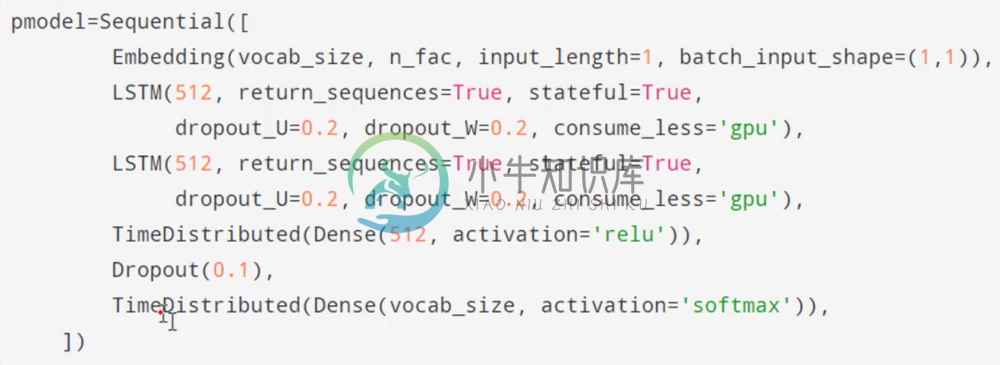
Let’s look at an example of a successful model Jeremy built to writing Nietzsche.
RNN Depth
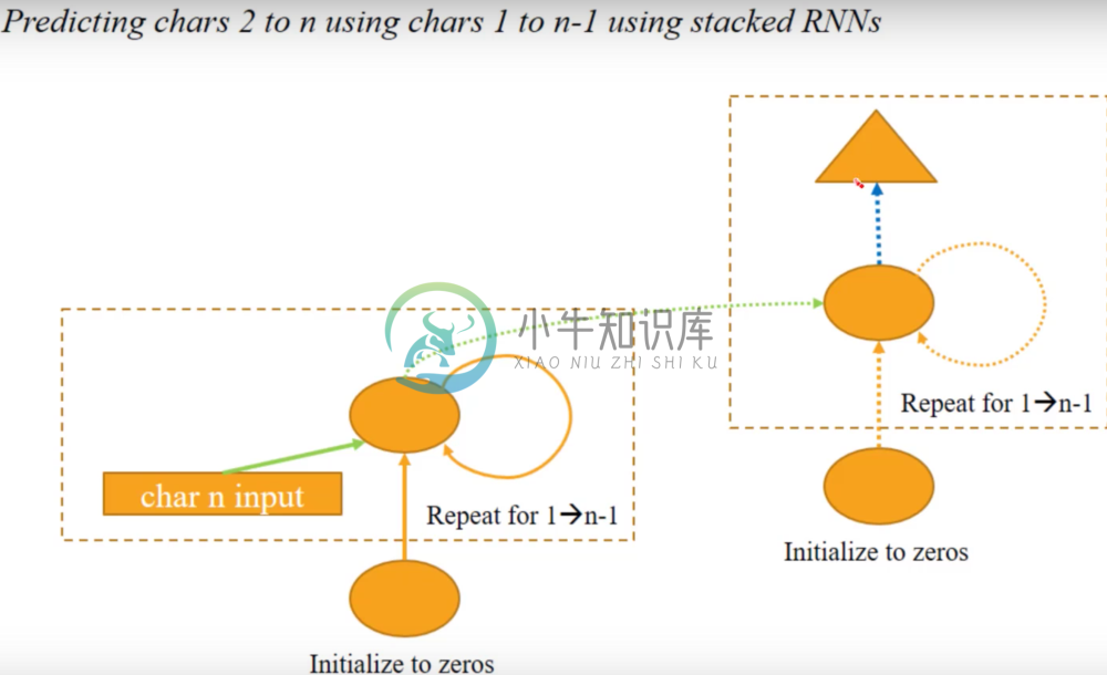
Notice that there are two sequential RNN’s, and they look like this:
The purpose of stacking RNN’s like this is that it allows to actually build a deep RNN, because now our inputs are going through multiple transformation prior to making an output, while still maintaining state. This of course gives us better results, as the structure of language is complex and a more flexible architecture will allow us to learn more.
Network Layers
Notice that we’ve also added dropout to our RNN’s, which has been shown to be a great way to regularize an RNN.
Our last addition was to add an extra dense layer before our final output. Notice that these dense layers are sitting within a layer called TimeDistributed(). Recall the output of our RNN layers in our sequential model from earlier; we had eight outputs, each with 256 activations. What we want to do is to apply the same weight matrix to each one of those outputs’ 256 activations; however, a standard Dense layer expects the inputs to be a flattened vector. Therefore, all the Time Distributed layer does is it creates as many copies of the layer inside it as there are outputs in your sequence, each sharing the same weight matrix, and applies it to each output. Anytime we’re returning a sequence of outputs in Keras, we’re going to have to use Time Distributed if we want to pass those outputs to a dense layer.
Training and Results
It’s also important to keep in mind that we want to reset our state at the end of each epoch. In other words, we only want to keep track of state throughout the entire corpus; once we restart it, we want to reset our state to zero.
Jeremy’s run_epochs(n) function velow does just this for n epochs.
We can see that after running just one epoch, our loss is atrocious and our output is correspondingly gibberish after feeding it a small sequence.
However, after running about 12 more epochs we can see that it’s starting to learn how to form words and even open chapters.
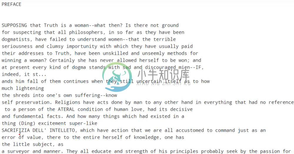
After training this overnight and feeding it a larger sequence to start with, we get the following.
This is quite impressive. It’s starting to say phrases that sound like something the author might actually say. In fact, we can actually see signs of overfitting in the presence of the phrase “SACRIFIZIA DELL’ INTELLETO”, which is ripped exactly from the text.
After playing around with various approaches, Jeremy found that the most successful technique was to simply apply batch normalization after the embedding layer. We can see the results of this on training below:
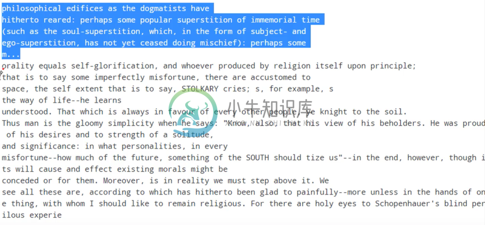
With batch norm, we’re decreasing our loss much faster. After training this model overnight, Jeremy achieved the following results given the highlighted seeding text:
This is really astounding We can see that it’s learned to put together some deep-sounding snippets such as “morality equals self-glorification”. It’s even learned to make sure to close quotes, even when that quote is formed along time ago. What’s even more astounding is that pretty much none of these phrases appear. All of these phrases were put together by the network itself, not plagiarized from the corpus. This indicates that we’ve successfully avoided overfitting.
These are impressive results given that we’ve only used character embeddings of 42 elements without pre-training on a corpus of only 600,000 characters.
One application for a model like this would be an auto-complete software that used this type of architecture to suggest the correct next word. More importantly, one could use this type of model for anomaly detection. Given a seeding sequence, a sophisticated model can predict what the next events should be. If the actual events deviate from the expected events significantly, then these can be flagged as anomalies.
Theano
Our next exercise will be to learn how to construct an RNN in pure Theano. The impetus behind doing this is so we can really understand what’s going on behind the scenes in Keras; this is important because as we start to build more complicated models it’s important to know how to debug and understand what’s going on in this lower level framework. More importantly, as we want to add more and more stuff on top of or into Keras, we’ll need to understand Theano because it is the language Keras is using behind the scenes. Therefore we need to understand Theano so we can extend Keras to suit our needs.
One-Hot Encoded RNN
Before we get started, it’s important to point out that so far in this lesson we haven’t one-hot encoded our categorical targets as we’ve done in the rest of this course. The reason we’ve been able to do that is we’ve been using sparse categorical cross-entropy as our loss function, which is able to take an integer target instead of a one-hot encoded vector and does the indexing into that vector directly. As with the motivation for using embedding layers, the reason why we want to do this is for resource efficiency; we might have hundreds of thousand of categories which would make one-hot encoding unwieldy.
However, in recreating our Keras model in Theano we’re going to use one-hot encoding to make it clear what’s going on. We’re also not using an embedding layer, so we’ll be one-hot encoding our inputs.
Here’s how our sequential model (no state) with one-hot encoding looks in Keras
When we fit this in the same way, we get the same answer as our prior model using embeddings/sparse categorical cross-entropy.
RNN in Theano
We are going to proceed by building the components of this RNN in Theano:
Variable Declaration
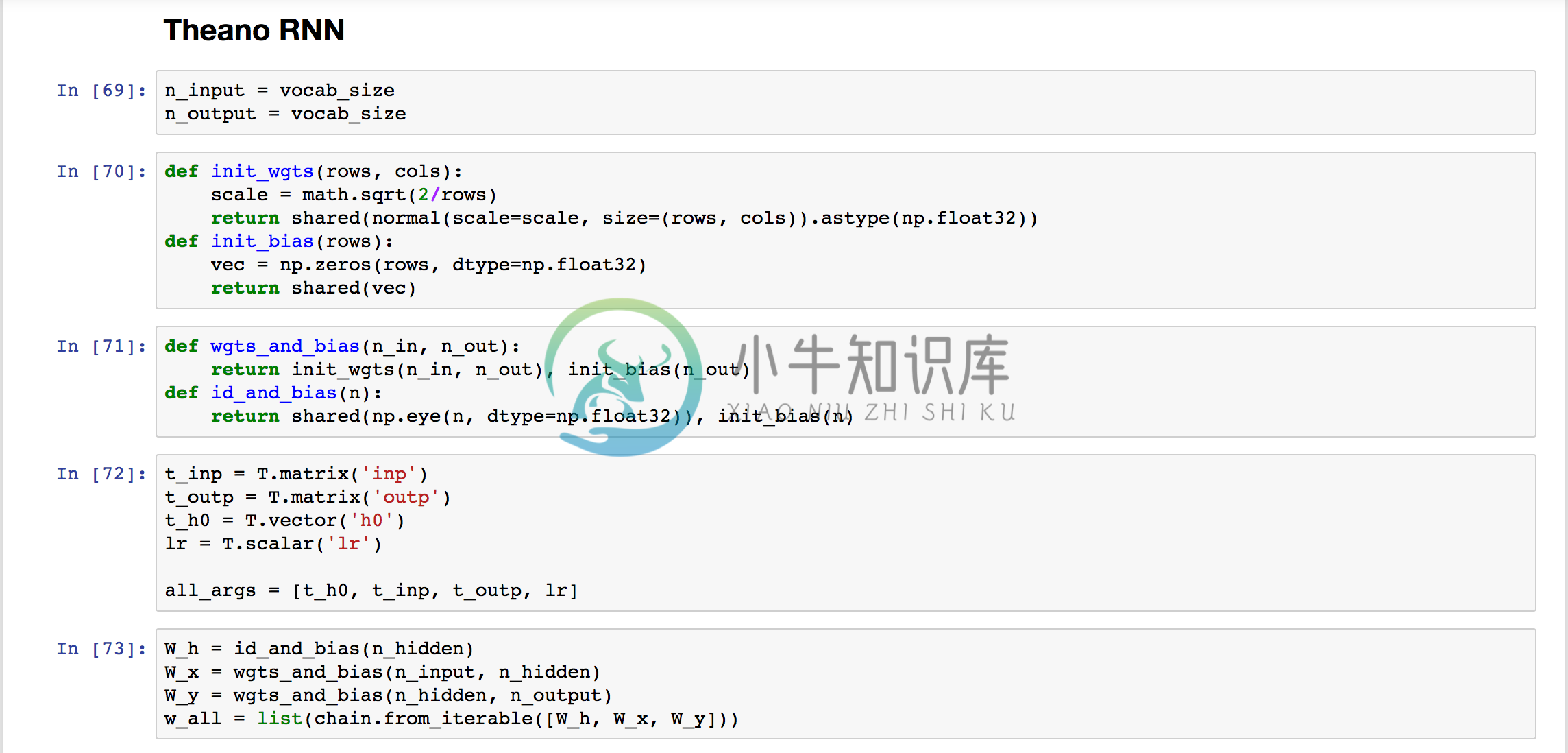
Notice the section above where we are defining variables. In Theano, we have to declare our variables before using them. We can see the individual calls for defining matrices, vectors, and scalars (and as we’ll see, operations). It is simply declaring that these are variables in Theano that we will assign values to later, and we collect them in a list called all_args.
The reason we declare these things is because Theano’s purpose is to provide a way for us to describe a computation that we want to do and compile it for the GPU where it’ll run the computations. By defining these variables and steps a priori, we’re building a computational graph that we can compile on the GPU, which will then be able to accept the data we want to give it in the future and perform the calculations we want to produce the output we desire.
Model Parameters
Next we manually initialize W_h as weights and biases to the hidden layer, W_x as weights and biases to the input layer, and W_y as weights and biases to the output layer. We initialize these values as we would expect, and we can see that in effect in the functions called to construct them (recall that we initialize the hidden weights to an identity matrix for an RNN).
However, when we return these values, we’ve wrapped them in a Theano function called shared(). This function simply tells Theano that this data is something that we’ll want to pass off to the GPU later for computation.
We can now combine all these parameters in a single list w_all as shown.
Step and Scan
Next, we’ll actually define to Theano what happens every time we take a single step in this RNN. It’s important to understand that on a GPU we can’t do a for loop; this is because by construction the GPU wants to be able to parallelize everything. By definition, a for loop can’t be parallelized because it can’t do the next part of the loop until the prior iteration has finished.
What we can parallelize is a scan operation, which calls some function for every element of some sequence and returns an output for each point. Then the next time the scan function is called, it’s going to provide the output of the previous call, along with the next sequence.
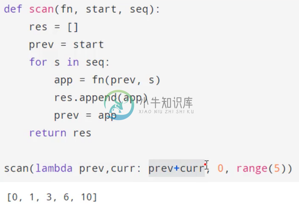
Below is an example of scan in python:
We can see that it takes as input a function, an initial value, and a sequence. Here, our function is simply adding two numbers together. The scan function applies this addition to the initial value, in this case zero, and the first element in the sequence. Next, it applies the same function to the output of the previous result and the second element of the sequence. It keeps doing this through the sequence, and the result is an array of cumulative sums.
It turns out that it’s possible to write a parallel version of this, and we can run it quickly on a GPU. Therefore our task is to turn an RNN into something we can run in a scan function.
The function we’re going to call is called step.
Let’s look at exactly what it’s doing. Inside the function call in the first line, we see that we’re transforming our input by our input layer and adding the biases, and then adding them to the transformed prior hidden state plus the hidden layer biases. That whole thing is then put through relu, our activation function, and we have our hidden layer activations. Next, we want to transform the hidden activations by our output weights plus the output bias, and then pass that through a softmax activation. Finally, we return our current hidden state, and our output.
Next, we declare the scan computation that we want to do. We do this by calling Theano’s scan function on our step function, and we feed as input/output the variables we declared earlier. We also give it all the other parameters that we’re going to be using, namely the weights.
Declaring the Function and Results
We’ve now described how to execute an entire sequence of steps for an RNN to Theano. When it runs, it’s going to return our hidden state and our output. We’ll define the rest below.
As we can see, the next step is to calculate our error using Theano functions, in this case categorical cross-entropy, given our step function outputs and our declared target matrix. We’ve now declared our error function.
Next, we’re also going to want to take the gradient of this error function with respect to all of the weights. This is easily done in Theano by simply calling T.grad(loss_function, parameters). Theano will then symbolically calculate all of the derivatives with respect to these parameters. Then we can update the parameters in correspondence with our learning rate.
Now that we’ve built our loss, gradient, and update function (which we’ve implemented with a dictionary), we’re ready to build our complete function in Theano with theano.function(). We give it as input: all of our arguments, which we defined earlier. As an output, it’s going to create an error function. After each step, it’s going to perform the weight updates.
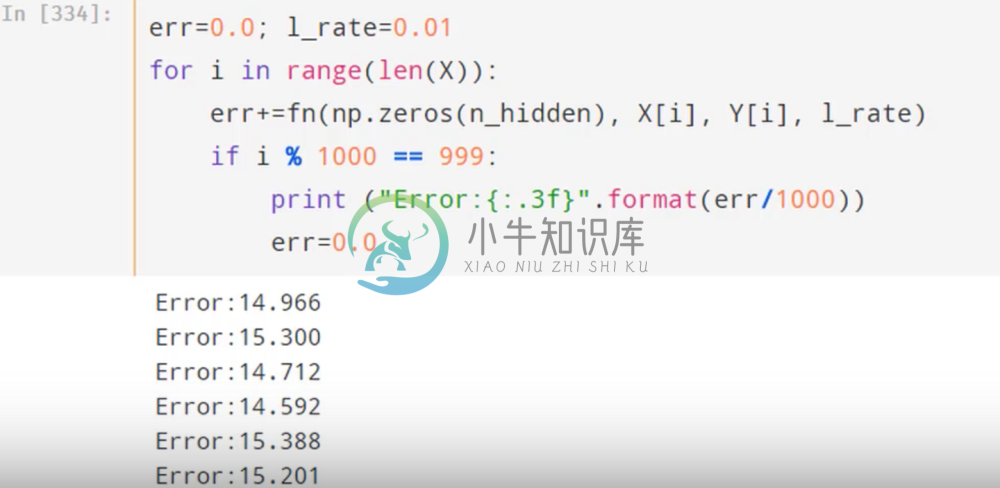
Let’s wrap this theano function in a for loop and call it for each individual element in our training data.
Here we are finally passing to our theano function the inputs that we defined earlier. Every time we call the theano function, it calculates the error and updates the parameters. Below, we’re printing the error after every thousand iterations, and we can see it start to improve. Note that what we’re doing here is stochastic gradient descent on a batch size of 1.
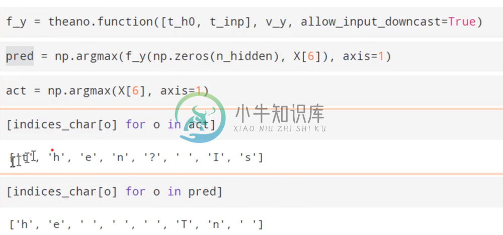
Now, we can make predictions:
In order to do this, we defined another Theano function that takes our hidden layers and word sequence as input and outputs the one-hot encoded response. We then find the index of maximal value to look up the word, and we can see the results.
We’ve now successfully built an RNN from scratch in Theano.
Next week, we’ll build an RNN by hand in numpy. This means we’ll have to calculate the gradient by hand.


