Lesson 4
This week’s links
- The lesson video
- Lesson 4 notes
- Lesson 4 Timeline
The notebooks:
- State Farm sample
- State Farm full
- Collaborative filtering with Movielens (dataset link below)
The spreadsheets:
Kaggle fish classification competition; also, a Fortune article discussing the background behind this competition
Information about this week’s topics
Collaborative filtering:
A fascinating deep dive into a Kaggle winners solution to an image classification problem
CNN Review
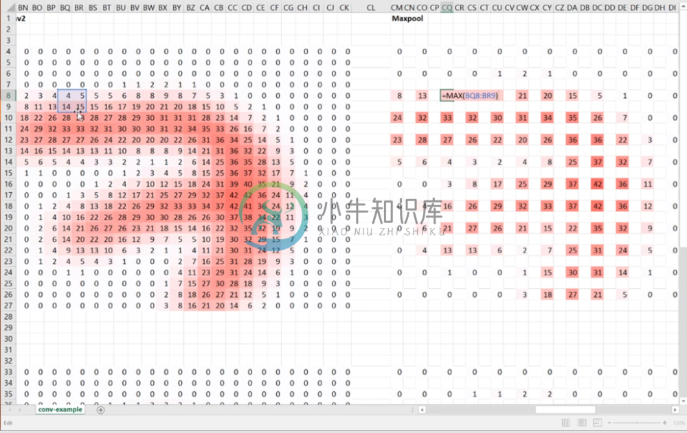
In our last lesson, we discussed convolutions and max-pooling in depth. As review, we’ll go over these concepts interactively through excel (see accompanying spreadsheet).
Convolutions Revisited
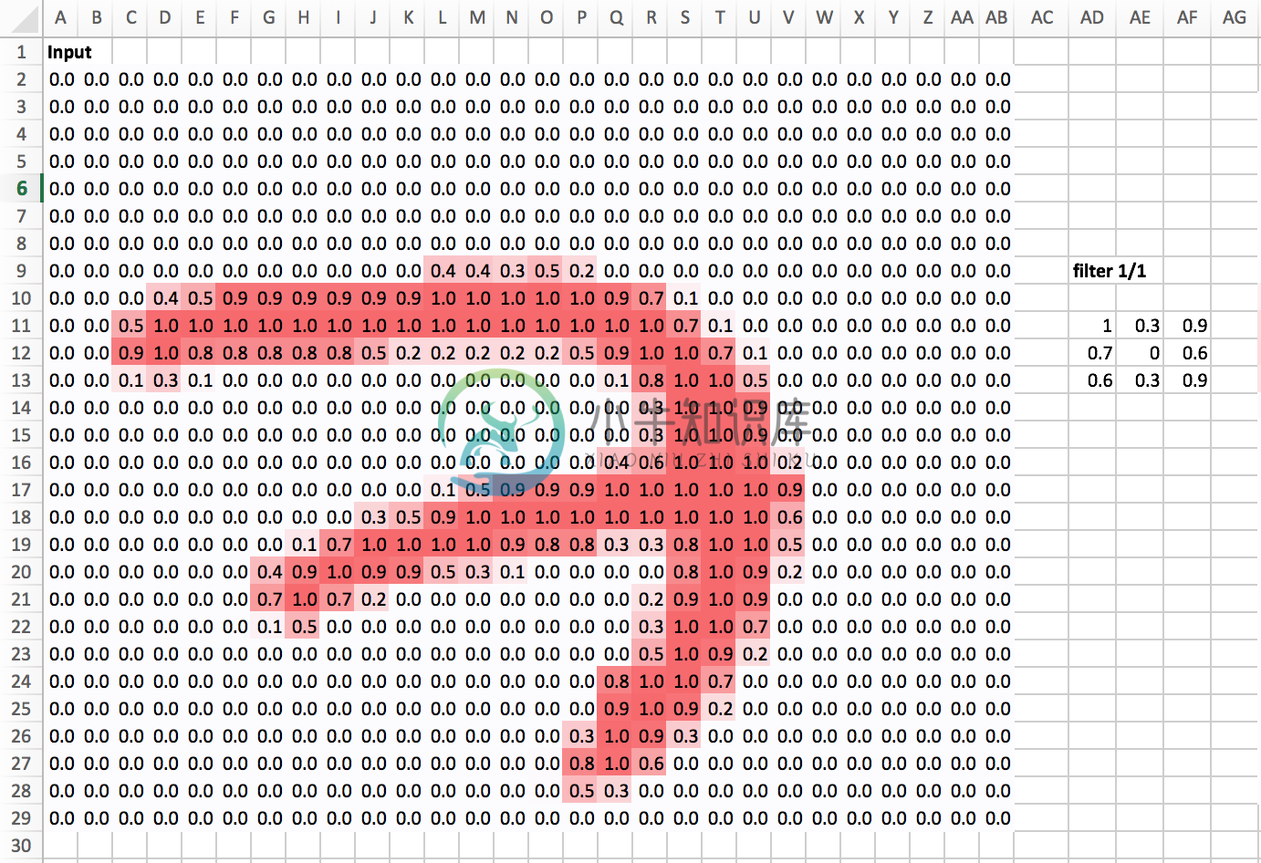
In this section we are going to explain the famous number 7 from first lecture:
The values on the left are the matrix that indicate the greyscale pixel values of our 7, while the 3x3 matrix on the right is a randomly generated 3x3 filter matrix that defines the convolution output.
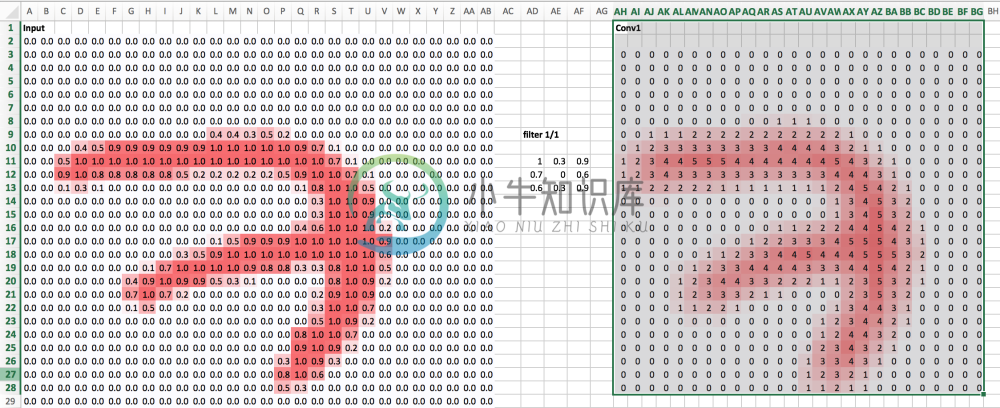
Let’s call the output of this filter Conv Layer 1 (denoted Conv 1). Recall from last week’s lesson that each pixel in Conv 1 is calculated by centering the 3x3 filter over the corresponding pixel in the original image, and taking the dot product over all overlapping values. Likewise, recall the usage of zero-padding; in order for Conv 1 to have the same dimension as our input image, we add a border of zeros around the original image to handle the convolutions at the edges and corners. Applying this function to every valid pixel in the padded original image, we produce Conv 1.
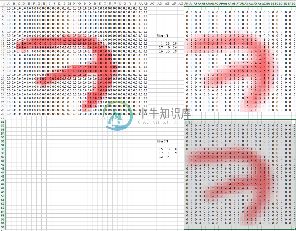
Likewise, we can see the output Conv 2 for a second randomly generated filter.
Remember that when we refer to a “Convolutional Layer”, we’re referring to a set of filters, and the output of the Convolutional Layer is the output of each filter applied to the original image. Therefore, in the above example, our convolutional layer has 2 filters, and therefore it’s output is a nxmx2 tensor, where nxm is the dimension of the original image (in greyscale). The third dimension is defined by the number of filters we’re applying, in this case 2, and is often referred to as “channel” or “depth”.
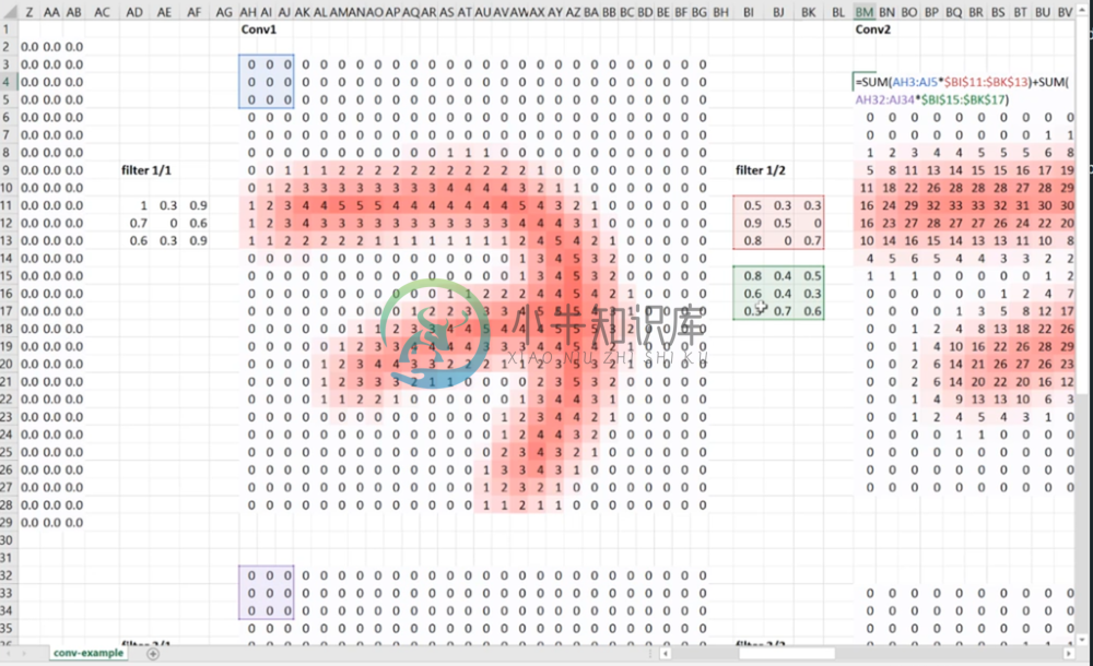
This new nxmx2 tensor is now the input for the second convolutional layer. Unlike the original image, we now have two channels to apply filters to. How should this be done? One might argue that we can simply apply a single 3x3 filter to both channels and add them up.
This can easily be done, but intuitively we know we shouldn’t do this. Remember, in CNN’s we think of filters at a high level as being able to identify certain features in the image. In our example, we are using two filters to identify two features from the input image, with the understanding that while these filters are initially random, back-propagation and gradient descent will eventually provide use with useful filters. Then the nxmx2 tensor outputted from convolution layer 1 can be thought of as two features extracted from the original nxm image. If in the next layer we apply the same filter to both channels and sum them up as the output, we’re using the same weights on both features. This makes for an inflexible architecture; in each filter in convolutional layer 2, we’re trying to force our weights to simultaneously work well at using the information from channel 1 and channel 2.
A smarter approach is to simply make our filters have as many channels as the input tensor. In our example, the filters in the second convolutional layer will have dimension 3x3x2. This allows us to define separate weights that act on channels 1 & 2 in the nxmx2 input, which in turn gives us greater flexibility in selecting weights in training that work best for channel 1 and channel 2 separately. After applying the filter channels to the corresponding input channels through the normal convolution operation, the final output is simply the sum of all of them.
In general, for any nxmxC input tensor to a convolutional layer, the filters will (typically) be 3x3xC, and the output of that layer will be nxmxF (given zero-padding) where F is the number of filters in that layer. This is why in most CNN architectures for color images, the filters in the first convolutional layer will be 3x3x3, as the input image has 3 channels (eg. RGB).
Max-Pooling:
Recall max-pooling from the previous lesson. The purpose of max-pooling is to simply reduce the resolution of our image. More generally we’re simply reducing the width and height dimensions of our intermediate convolution outputs, as this allows us to employ more filters while maintaining computational integrity. In addition, max-pooling forces our filters to start looking at larger spaces of the image.
In our example here, we’ve done 2x2 max pooling. All this does is replace each distinct 2x2 subsection of the image with a single pixel, defined as the maximum pixel from the original 2x2 area.
Dense Layer:
Finally, after our convolutions and max-pooling, we employ dense layers. In our example, we initialize two nxm random matrices, one for each channel from our convolution output, and sum the corresponding dot products. We could generalize this to multiple outputs by increasing the depth of these random weight matrices accordingly.
Of course, once we’ve initialized these weights amongst these filters and dense weight matrices, we update them through calculating partial derivatives with respect to a particular loss function as we’ve learned already, and descend down the gradient.
We know that there are of course more pieces in CNN architecture including non-linear activations, batch normalization, and dropout, but this should hopefully address any lingering questions on how convolutions, max-pooling, and dense layers work.
Optimizers Explained:
In this section, we explain a variety of different optimization techniques, which alter the basic approach to gradient descent. These techniques are used to help improve the arduous and sometimes inefficient task of adjusting learning rates for effective optimization. We’ve already discussed standard and stochastic gradient descent already, so we’ll skip to the new material. If you’re still uncomfortable with sgd, we suggest playing around with Jeremy’s sgd spreadsheet to help solidify your understanding.
Learning Rate
The rate at which we update parameters through gradient descent is determined by the learning rate. This can be thought of as the size of the “step” we take down the gradient in the hypersurface defined by our loss function. In general, standard and stochastic gradient descent employs a constant learning rate. However, this can cause a number of issues during training:
- If the learning rate is too small, the optimisation will need to be longer than may be necessary. In terms of step size, a small learning rate means our steps our too small and we may never reach a feasible optimum in reasonable time.
- If the learning rate is too big then the optimisation may be unstable. In terms of step size, this means are steps may be too large, and we might step over potential optimums or even bounce out of an optimum.
- The optimisation may get stuck in an unsatisfactory local minima, or other challenging areas like a saddle point.
The learning rate can be manually adjusted throughout the training process to improve performance, but this is a very ad-hoc methodology that doesn’t really use any of the information gained during the learning process. A better approach is to use some of the information about the loss function we’re optimizing during training, and modify our learning rate to reflect that.
Momentum
For NN’s,the hypersurface defined by our loss function often includes saddle points. These are areas where the gradient of the loss function often becomes very small in one or more axes, but there is no minima present. When the gradient is very small, this necessarily slows the gradient descent process down; this is of course what we desire when approaching a minima, but is detrimental otherwise. Momentum is intended to help speed the optimisation process through cases like this, to avoid getting stuck in these “shallow valleys”.
Momentum works by adding a new term to the update function, in addition to the gradient term. The added term can be thought of as the average of the previous gradients. Thus if the previous gradients were zig zagging through a saddle point, their average will be along the valley of the saddle point. Therefore, when we update our weights, we first move opposite the gradient. Then, we also move in the direction of the average of our last few gradients. This allows us to mitigate zig-zagging through valleys by forcing us along the average direction we’re zig-zagging towards.
Dynamic Learning Rates
Momentum does well at decreasing optimization time for some parameters overall, but we still often find that certain parameters can take along time. A better approach is to dynamically adjust the learning rate factor for each parameter, utilizing information gained from the optimization process.
Adagrad
Traditionally the learning rate is constant for all parameters in the model. Adagrad is a technique that adjusts the learning rate for each individual parameter, based on the previous gradients for that parameter. Essentially, the idea is that if previous gradients were large, the new learning rate will be small, and vice versa.
The implementation looks at the gradients that were previously calculated for a parameter, then squares all of these gradients (which ignores the sign and only considers the magnitude), adds all of the squares together, and then takes the square root (otherwise known as the l2-norm). For the next epoch, the learning rate for this parameter is the overall learning rate divided by the l2-norm of prior updates. Therefore, if the l2-norm is large, the learning rate will be small; if it is small, the learning rate will be large.
Conceptually, this is a good idea. We know that typically, we want to our step sizes to be small when approaching minima. When they’re too large, we run the risk of bouncing out of minima. However there is no way for us to easily tell when we’re in a possible minima or not, so it’s difficult to recognize this situation and adjust accordingly. Adagrad attempts to do this by operating under the assumption that the larger the distance a parameter has traveled through optimization, the more likely it is to be near a minima; therefore, as the parameter covers larger distances, let’s decrease that parameter’s learning rate to make it more sensitive. That is the purpose of scaling the learning rate by the inverse of the l2-norm of that parameter’s prior gradients.
The one downfall to this assumption is that we may not actually have reached a minima by the time the learning rate is scaled appropriately. The l2-norm is always increasing, thus the learning rate is always decreasing. Because of this the training will reach a point where a given parameter can only ever be updated by a tiny amount, effectively meaning that parameter can no longer learn any further. This may or may not occur at an optimal range of values for that parameter.
Additionally, when updating millions of parameters, it becomes expensive to keep track of every gradient calculated in training, and then calculating the norm.
RMSProp
RMSPRop is very similar to Adagrad, with the aim of resolving Adagrad’s primary limitation. Adagrad will continually shrink the learning rate for a given parameter (effectively stopping training on that parameter eventually). RMSProp however is able to shrink or increase the learning rate.
RMSProp will divide the overall learning rate by the square root of the sum of squares of the previous update gradients for a given parameter (as is done in Adagrad). The difference is that RMSProp doesn’t weight all of the previous update gradients equally, it uses an exponentially weighted moving average of the previous update gradients. This means that older values contribute less than newer values. This allows it to jump around the optimum without getting further and further away.
Further, it allows us to account for changes in the hypersurface as we travel down the gradient, and adjust learning rate accordingly. If our parameter is stuck in a shallow plain, we’d expect it’s recent gradients to be small, and therefore RMSProp increases our learning rate to push through it. Likewise, when we quickly descend a steep valley, RMSProp lowers the learning rate to avoid popping out of the minima.
Adam
Adam (Adaptive Moment Estimation) combines the benefits of momentum with the benefits of RMSProp. Momentum is looking at the moving average of the gradient, and continues to adjust a parameter in that direction. RMSProp looks at the weighted moving average of the square of the gradients; this is essentially the recent variance in the parameter, and RMSProp shrinks the learning rate proportionally. Adam does both of these things - it multiplies the learning rate by the momentum, but also divides by a factor related to the variance.
Eve
Eve is an extension of Adam that also keeps track of the change in loss function, and incorporates this difference into the learning rate. You can peruse the details [here], but essentially Eve increases the learning rate when there is little to no change in the loss function, and decreases it when the loss function fluctuates.
This can be helpful: when the loss function is barely changing, it could be indicative of being stuck in a shallow plain in the hypersurface, and increasing the learning rate may push us through it. Like wise, if the loss function is fluctuating wildly, it could mean that we’re bouncing around a minima, and we should decrease the learning rate.
However, there’s an obvious flaw in Eve; when we approach a minimum, we expect the loss function to stop changing. In this scenario, Eve wants to increase the learning rate, which can bounce us out of our minimum.
Jeremy’s Dynamic Learning Rate
In this lesson, Jeremy offers his own approach to dynamic learning rate annealing. In his approach, he constructs a system where the learning rate always goes down, and instead of relying upon the oft bumpy loss function, we rely on the average sum of squared gradients.
The idea is to compare the ratio of the sum of squared gradients between each epoch. If we are approaching a minimum, we expect the sum of squared gradients to always decrease from one epoch to the next. If the sum of squared gradients ever increases, we can consider that a strong indication that we’ve bounced out of the area of interest.
In the accompanying notebook, Jeremy demonstrated this approach by simply modifying his Adam spreadsheet to decrease the learning rate by a factor of four if the sum of squared gradients doubles from one epoch to the next. The idea is to hopefully automate the learning rate annealing process.
Insights from Jeremy’s Approach to Kaggle’s Statefarm Competition
In lesson 4, we go over Jeremy’s entry to the Statefarm Distracted Driver Detection competition. Here we discuss some insights revealed in his submission.
Testing on Samples
By this point, we’ve mentioned several hyperparameters such as dropout rate and learning rate. Loosely speaking, a hyperparameter is a parameter used in a model that is not modified through training; rather it is chosen a priori and modified by the user to optimize the desired outcome.
As mentioned before, it is good practice to tune hyperparameters and modify architectures on a random sample set of the overall training data, as this reduces computational time drastically. Fortunately, we typically find that our sample set is general enough to ensure that the tuning and design choices made on the sample set work well on the entire set.
Input Batch Normalization
As discussed last lesson, it’s good practice to always normalize our inputs. Instead of manually calculating averages and variances across the entire training set, a much simply approach is to start your Keras model with a Batch Normalization layer. This will handle the input normalization for you, and is a good default starting point.
Linear Model
We start with a simply linear model in Keras to see how we might tune hyperparameters in practice.
Upon compiling and fitting, we find that our training and validation accuracies are very low. While we would not expect a linear model to perform as well as typical architectures, here are still over a million parameters so we do expect some performance. Therefore, underfitting is likely not the problem
A more likely reason is that the learning rate is too high, and we jump too far at the start of training.
Often times, there are reasonable solutions to our optimization problem that are very easy to find. For example, in the Statefarm competition we try to classify each picture into one of ten classes. A plausible solution is for our model to simply predict the same class every time. But of course this isn’t a minimum we’re interested in.
The solution to avoid this is to start with a very low learning rate to avoid jumping to an undesirable minimum, and then increase once we’re no longer at risk of getting stuck there.
Architectures
It’s also useful to test the effectiveness of different architectures and data augmentation techniques on a sample. With Statefarm, we employ a CNN for image recognition, and in the lecture we see how even a very simple CNN can get a vlidation accuracy of 67%.
Tuning Data Augmentation
To date, there is no rigorous approach to finding optimum parameters for data augmentation. We recommend scanning values for data augmentation techniques separately, selecting those that produce the best results upon implementation, and combining them. This tuning can easily be done on a sample.
Regularization:
Regularization, however, cannot be tuned on a sample. Recall that regularization attempts to prevent overfitting by attempting to make our network generalizable in training. Necessarily, a small sample will need more regularization to generalize to unseen data than a large training set, because the training set will necessarily contain more of the variation inherent in the population.
Semi-Supervised Learning
In the Statefarm dataset, we have a very large test set of 80,000 images, compared to only 20,000 images in the training set. That’s a big difference, and it seems a shame that we’re unable to learn more information from the test set.
It turns out we can use the unlabelled data to help us gain more understanding of the population structure in general. This is what’s known as Semi-supervised learning.
Psuedo-labeling
One remarkably simple approach to utilizing unlabelled data is known as psuedo-labeling. Suppose we have a model that has been trained on labelled data, and the model produces reasonably well validation metrics. We can simply use this model then to make predictions on all of our unlabelled data, and then use those predictions as labels themselves. This works because while we know that our predictions are not the true labels, we have reason to suspect that they are fairly accurate. Thus, if we now train on our labelled and psuedo-labeled data we can build a more powerful model by utilizing the information in the previously unlabelled data to better learn the general structure.
One parameter to be mindful of in psuedo-labeling is the proportion of true labels and psuedo-labels in each batch. We want our psuedo-labels to enhance our understanding of the general structure by extending our existing knowledge of it. If we allow our batches to consist entirely of psuedo-labeled inputs, then our batch is no longer a valid representation of the true structure. The general rule of thumb is to have 1⁄4-1⁄3 of your batches be psuedo-labeled.
Collaborative Filtering:
In this section, we’ll start to move on from CNN’s towards deep learning in Natural Language Processing (NLP), and we begin by introducing collaborative filtering.
Recommender Systems
A recommender system is something that predicts who is going to like what, and by how much. There are two main ways to build recommender systems:
- Using meta-data such as surveys to filter results, such as showing sci-fi films to a Netflix user that has indicated they like sci-fi through some form
- Using collaborative filtering, which gives results that match the preferences of users that are similar to you.
In a movie recommender system, collaborative filtering will look for users that have rated the same movies you have, and rated them in a similar way.
It turns out that with a large enough data set, collaborative filtering is much more powerful than the meta-data approach. In fact, it has been shown that adding meta-data to collaborative filtering approaches had no effect.
The dataset we’ll be using in exploring collaborative filtering is the Movielens Dataset.
Movielens Spreadsheet
[](http://wiki.fast.ai/index.php/File:User_ratings.png “Enlarge”)
To obtain a firm grasp of collaborative filtering, we highly recommend you play around with the accompanying Excel spreadsheet. We go over it briefly here.
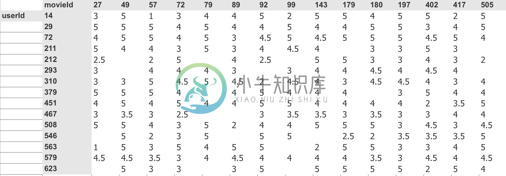
The Movielens dataset contains user ratings for different movies. As an exercise, we’ve taken the top fifteen users and movies, and we can see their rating here.
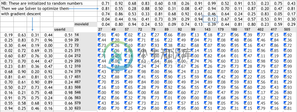
Collaborative filtering is an approach that learns from this sort of data to make predictions for new users, and this is done by constructing an embedding for every distinct mover and every distinct user. These embeddings are simply vectors whose elements describe an as of yet unknown quality or feature. If we take the dot product for each user/movie embedding pair and call it that user’s rating for that movie, we can now train the elements of each embedding as parameters in a gradient descent optimization problem, where the actual ratings are used as the true labels. In the lecture, we can see we’ve achieved pretty good results using such a simple idea.
[](http://wiki.fast.ai/index.php/File:C_filt.png “Enlarge”)
One thing we have not accounted for yet is bias. In this context, we can think of bias as something that might describe whether or not a user in general likes movies more than others, or whether some movies are more popular than others. We can include this by modifying our collaborative filtering process to include bias terms for each user and movie, which are simply added on to the dot product. These bias terms are also treated as parameters in training, and optimized in gradient descent. We find after training that our result here is better than without bias, as expected.
In our example, we’ve created embeddings with five elements, which we call latent factors. As an example, some possible features these latent factors may represent for a movie embedding are things like whether the movie is a blockbuster, if it’s funny, etc. But more often than not we don’t actually know exactly what attributes these factors are describing, only that through gradient descent we have learned these to be the most useful at predicting user ratings. We often employ visualization techniques to get a sense of what is being described.
In regards to retrieving these latent factors given a user or movie ID, Keras uses something called an Embedding Layer that looks up the appropriate embeddings given an id, and handles the training of said factors.
While our simple dot product approach gave decent results, we can do much better using a Neural Net. If we concatenate the latent factor embeddings given a movie and user id, we just have a vector, and we can simply train a neural network based on this input to our known ratings. Even a very simple architecture has been shown to achieve much better results than state of the art.


