Lesson 5

Tips to get 98.94 acc on Cats and Dogs Redux 00:00:00

[TODO] Summarize the model, techniques and hyperparameters

Introducing Batch Normalization into a Pre-Trained Model 00:01:55

Before we move on from CNN’s, we wanted to talk about how we can introduce Batch Normalization into a pre-trained convolutional neural network that doesn’t already have it.

Batch Norm Review

As a reminder, batch normalization has become something of a standard now because it increases training speed and tends to reduce overfitting. This makes it desirable in any CNN architecture, as it lets us avoid relying too heavily on dropout to reduce overfitting; this is a good thing because dropout is a loss of data, which is always best to mitigate.

Recall that batch normalization works by first normalizing the output of a previous activation layer by subtracting from each output the batch mean and dividing by the batch standard deviation. Next, the normalized outputs are “denormalized” by multiplying by a “standard deviation” parameter (gamma) and adding a “mean” parameter (beta). In other words, the normalized outputs are scaled and shifted by trainable parameters. This allows us to normalize the activations to increase the stability of the neural network, while allowing gradient descent to undo this normalization in a way that minimizes our loss function.

Using Batch Norm with VGG

Frequently throughout this course we have fine-tuned the pre-trained VGG 16 model to do various image classification tasks with great success. However, VGG lacks batch normalization, because at the time it was created batch normalization didn’t exist. Therefore, it’s reasonable to ask whether or not we can improve VGG’s performance by updating it’s architecture to include batch normalization.

Let’s now consider the challenge in introducing batch normalization to a pre-trained network like VGG. Consider that in consecutive layers, the weights are trained to be optimal given the output of the prior activation layer. Therefore, if we normalize the activation outputs and shift/scale by some randomly initialized parameters, the weights in the next layer are no longer the optimal transformation for these new inputs. This disruption will cause chaos in gradient descent, and it would take a considerable amount of training to get back to an optimal state, which nullifies the purpose of using a pre-trained network.

The solution is quite simple; we should initialize the scaling and shifting parameters to be exactly the standard deviation and mean of the inputs. This means that in our first pass through, the normalization transformation is effectively undone, and the next layer’s weights are still optimal. Then, back-propagation will update the scaling and shifting parameters in an appropriate matter. In other words, this method avoids the destabilization that randomly initialized batch norm parameters cause; it does this by starting in a stable state, and allowing gradient descent to inform the network how these parameters should change to minimize the loss function.

As a result of simply introducing batch normalization to VGG, Jeremy was able to achieve an accuracy of 98.95% for the Dogs vs. Cats data set, which is better than the first place result in that competition.

Collaborative Filtering 00:10:00

Bias Model

Recall our collaborative filtering task we started last week. Given a matrix of user ratings for movies, we had defined random embeddings for each user id and movie id. These embeddings are simply vectors, one each for every unique user/movie id. We also defined user and movie bias parameters, also unique to each id. Finally, we built a model wherein the predicted rating for a movie given a user was defined as the dot product between the user and movie embeddings, plus the two respective bias parameters. We then used gradient descent to find the embedding elements (and biases) for each user and movie that minimized our loss function, using the actual user ratings as the true targets. This bias model gave us decent results.

In fact, it turns out that we can achieve a relatively state-of-the-art model with this simple bias approach by simply adding regularization. In this particular case, an L2 weight regularizer was added to our loss function. Recall that the L2 norm is simply the sum of squares; therefore the purpose of adding the L2 weight regularizer to our loss function is to avoid large weight values when possible. After regularization, this bias model achieved a loss of 0.7979, which is better than the academic state-of-the-art.

Adding regularization to loss function 00:13:45

Analyzing Parameters 00:15:40

The obvious application for this model is for predicting user ratings, which we can then use to inform a UI how to display results to a particular user. However, there is additional information we can gain from the learned parameters themselves.

Bias

The learned biases are particularly revealing in telling us what movies are good and bad; unlike an average rating for a movie, the bias parameter takes into account the aspects of each user that rates a movie. Therefore, unlike the mean, which is susceptible to things like users who rate more favorably, who are more critical, etc., the bias term is independent of all of that noise.

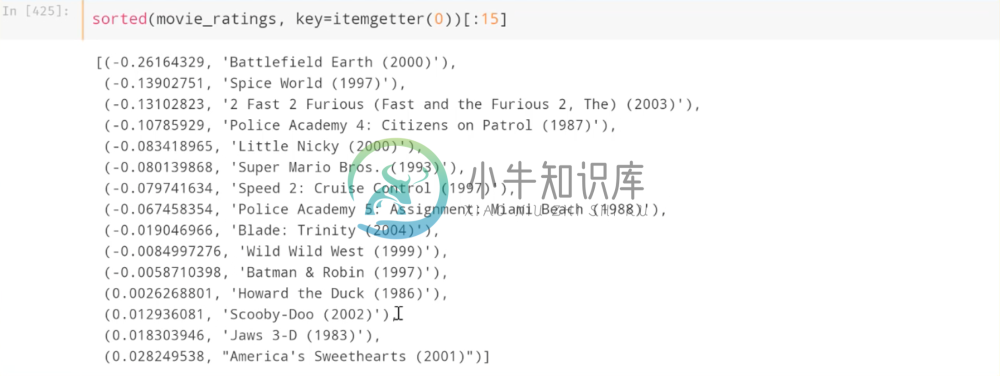
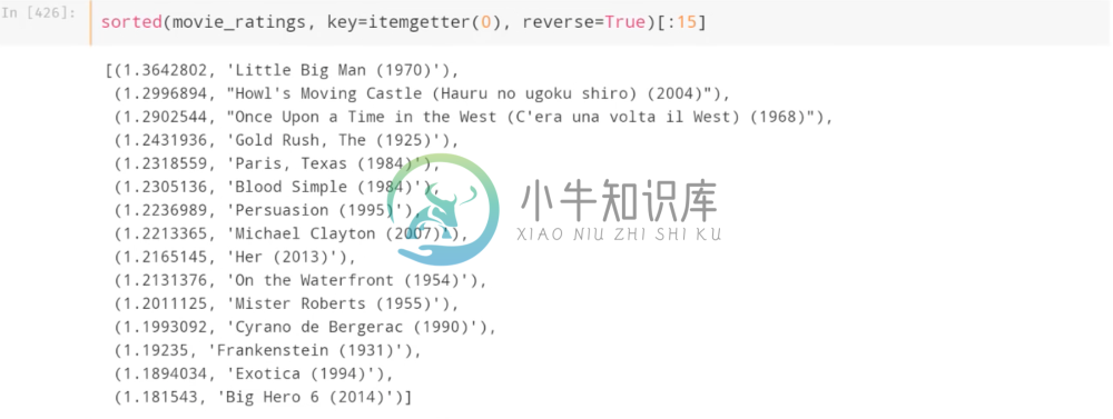
Below, we’ve taken the top 2000 movies in our dataset and sorted by lowest and highest biases.

These are all fairly atrocious movies, so it would seem these parameters have done a good job here.

These results also aline with our expectations in general.

Latent Factors & PCA

In collaborative filtering, the elements in the embeddings are often referred to as latent factors, and last time we had assumed that each one of these latent factors represented some aspects about a user or movie

Latent factors can be challenging to interpret. In our example, we had 50 latent factors. We use PCA to extract the first three principle components that capture the most information out of these 50. We can then observe the opposite ends of these components by value, and attempt to understand what information they’re conveying.

As an example, we can see below the highest and lowest values for our first principle component.

This component seems to capture a movie “classic” status. At one end, we see movies such as The Godfather, Pulp Fiction, Toy Story, and Ferris Bueller’s Day Off, which are all movies that widely considered to be cinema classics in their respective genres and eras. Meanwhile, the other end includes movies such as Robocop 3 and Judge Dredd, movies that likely don’t have much in the way of any sort of status other than less-than-stellar.

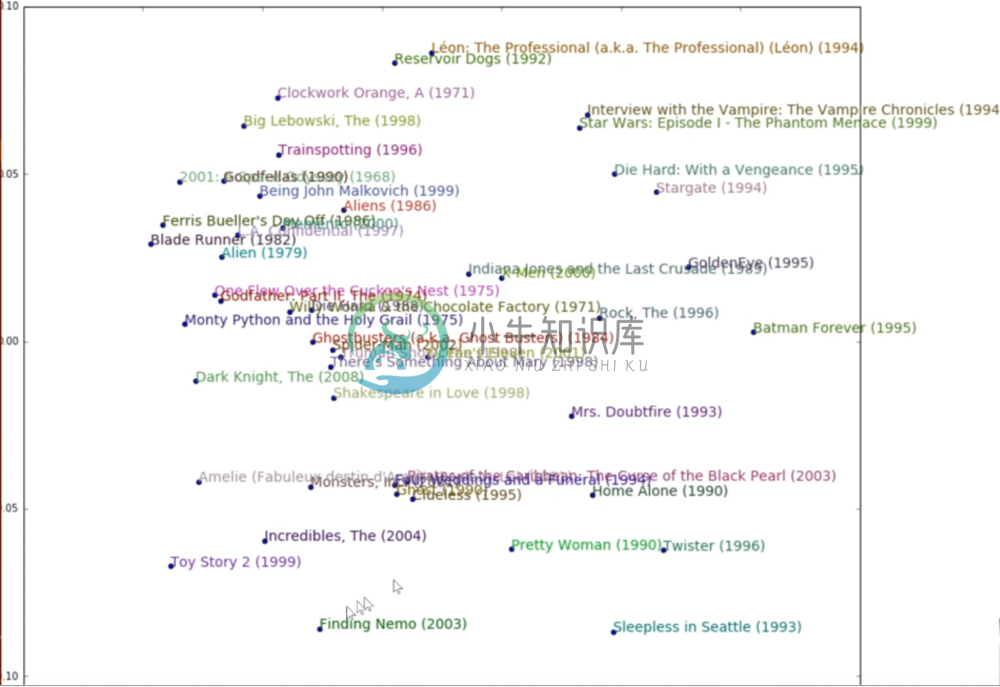
What’s useful about this type of principle component analysis on our latent factors is that it helps with visualization. Below we’ve plotted our movies with the first principle component on the x axis, and the third principle component on the right. The third principle component seems to describe the violence or intensity of a movie.

With this visualization, we can see the classic films on the left, and the more Hollywood-esque films on the right. Further, the more violent films are near the top, and the less violent are near the bottom. As an example, we can find A Clockwork Orange at the top left, which is a Kubrick classic, yet also an intensely violent film.

The purpose of these visualizations and analyses is to suss out inferences from these learned latent factors. We have no idea what these latent factors are after training; gradient descent selected them, and therefore it’s necessary to use these approaches to understand what the model is telling us.

Keras Functional API 00:23:40

So far in this course we have been using Keras’ sequential API for building our models. This has worked perfectly fine with the models we’ve built so far, but today we’ll begin looking at the functional API, which gives us more control over designing our architecture.

Below is an example of a fully connected neural network using the functional API. Notice that at each step, we define the next layer, and then immediately call the output of the previous layer. Finally we can build the model by selecting the appropriate input and output layers and compiling.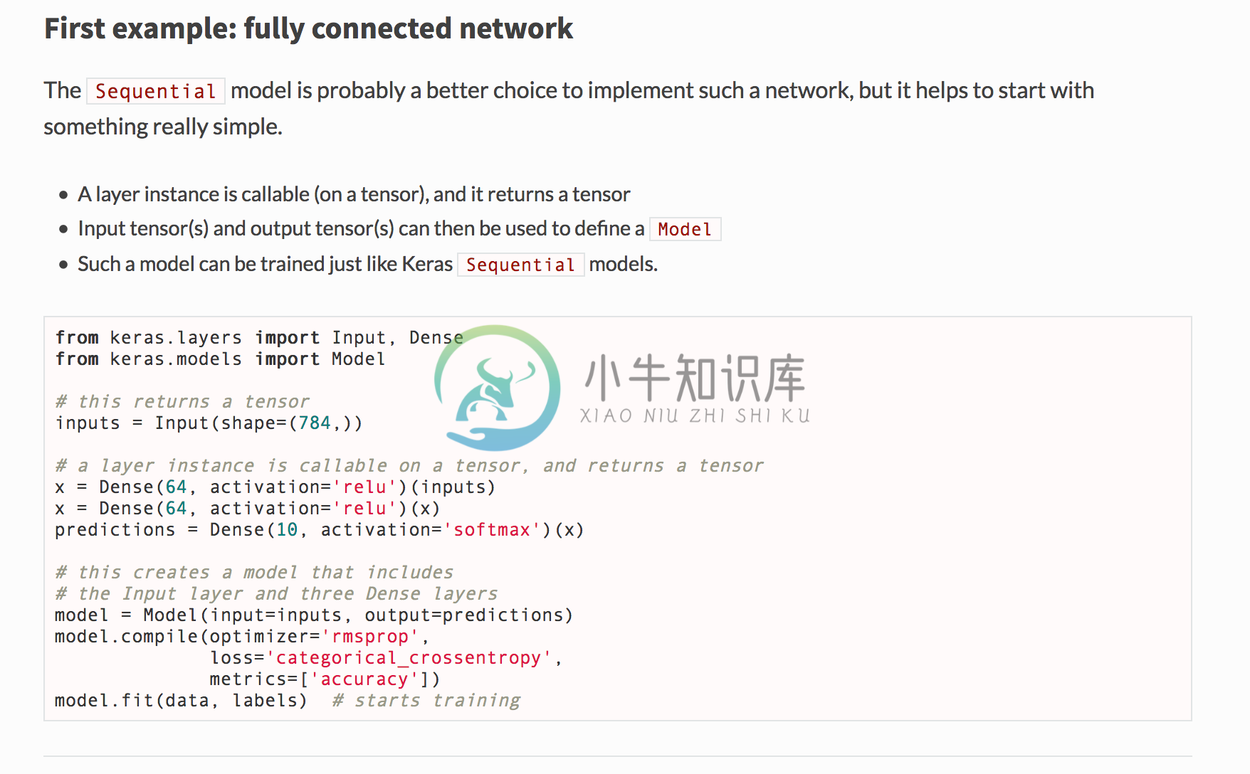

You can read more about it here.

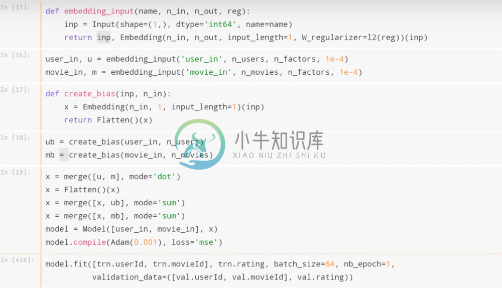
We can see the utility of the functional API in building a model for our collaborative filtering, which would be incredibly difficult with the sequential API.

Here, we’ve built four models, the embeddings and biases for the users and movies respectively. The functional API allows us to take the dot product of the embedding models and add the respective biases. It also allows us to then build the model such that it takes two inputs, and outputs our predicted ratings. This would be extremely difficult with the Sequential API, and as we can see the functional API makes this very natural and intuitive.

As we continue to study more exotic architectures, we’ll be utilizing the functional API more and more. One obvious use case of the functional API is that it can allow us to add meta-data to the CNN models we’ve studied so far. As an example, we might find it useful to add the image size as a feature to a CNN; the functional API allows us to do that.

An Aside on Embeddings Functions

One might reasonably wonder what the difference is between using an embedding of N-element vectors, rather than using one-hot encoding for each individual index and applying a weight matrix. The answer is, they’re exactly the same. If you have M indices, and you want to train N parameters for each index, then using a one-hot-encoding approach is simply multiplying the NxM weight matrix with the Mx1 one-hot encoded vector. The weights you would learn would be exactly the same as those in an embedding function.

The difference is simply that an embedding is just a look-up function. Multiplying an NxM weight matrix with a one-hot encoded vector simply returns the i-th column of the weight matrix, where i is the non-zero index. Therefore it’s a waste of computational time to perform such a calculation, so an embedding function just looks it up.

Natural Language Processing 00:34:00

While collaborative filtering is important, the primary reason we have covered it is to introduce the concept of embeddings. In reality, what we’re really interested in is the application of embeddings to Natural Language Processing (NLP). The purpose of fast.ai and this course is to introduce the shape and structure of these common problems in the hope that you will be able to take these frameworks and apply them elsewhere. One possible application of NLP with deep learning is building a diagnostic tool that can make predictions based off of patient medical history.

Sentiment Analysis

We’ll begin our dive into NLP by tackling a classic problem in the field, which is Sentiment Analysis. The goal of sentiment analysis is straightforward: given text, can we predict the sentiment expressed within it (i.e. negative, neutral, positive).

Keras comes with a well known data set for sentiment analysis, the IMDB Sentiment dataset, which consists of movie reviews and their respective sentiments. It’s been thoroughly tested and researched upon, and a good paper about it can be found here.

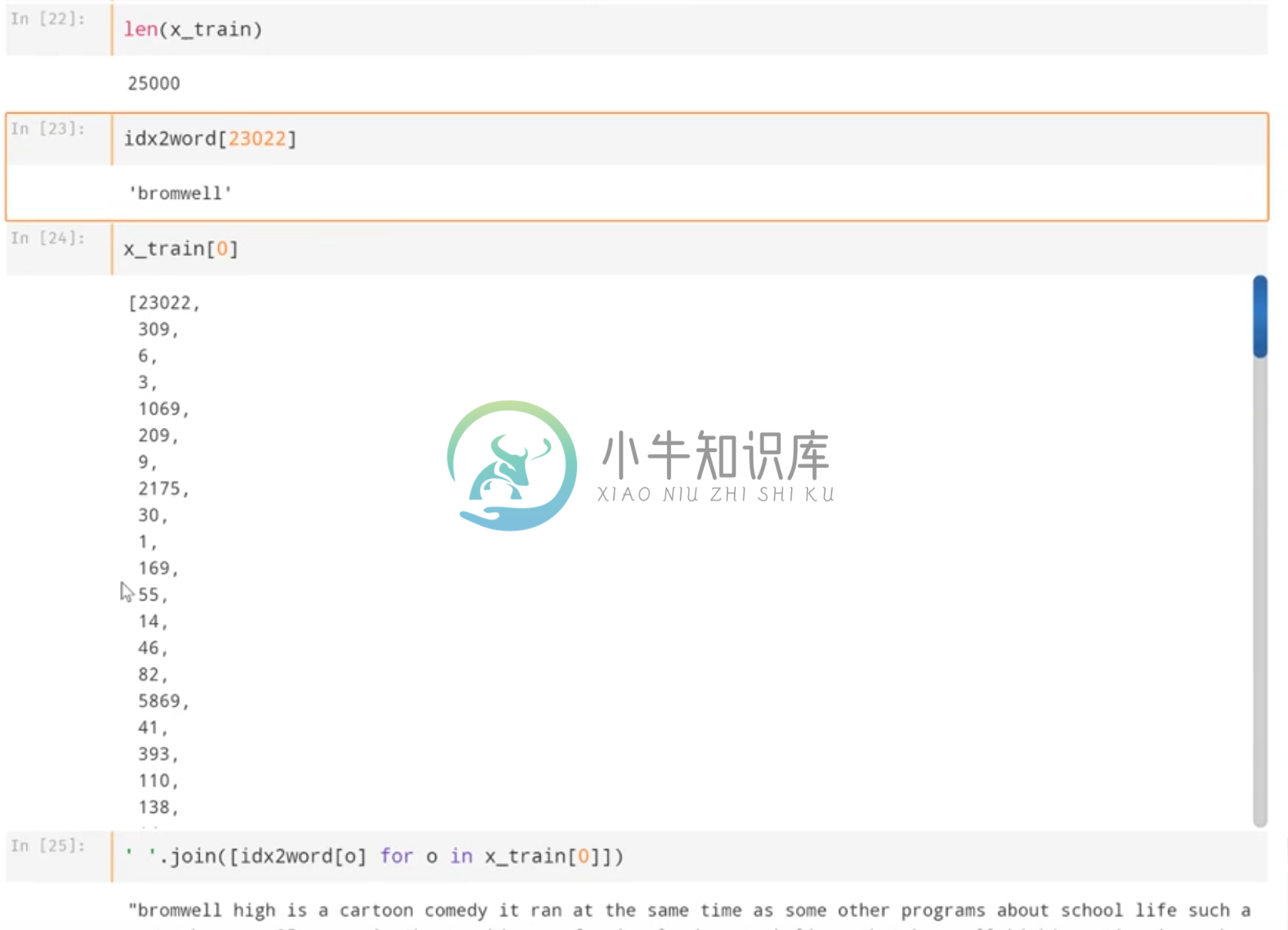
The dataset contains 25,000 movie reviews. Each review is a vector of word indices in the order the words are written; the word itself can easily be looked up using the index. The target is also provided, with a 1 as positive sentiment and a 0 as negative.

Our goal is to take these reviews and determine if they are positive or negative.

We can start by making this task simpler. One logical step to make is to truncate the vocabulary to some number of the words that occur most often in the corpus. This is sensible because infrequent words are not going to give us much useful information since there are not a lot of examples of them to train on. Further, there are a lot more infrequent or one-off words than there are frequent words. Therefore, by getting rid of these useless words we also drastically diminish the number of parameters for our network, which of course diminishes it’s complexity and makes our lives easier. We don’t want to lose the information on the presence of these rare words however, so rather than get rid of them we simply treat them all as if they were the same word by setting them to the same index.

Fortunately, the index table in Keras is ordered by frequency, which makes it easy to do this. In our case, we want to truncate our vocabulary to 5000 words; we can easily do this by retaining all indices less than 5000, and setting all indices greater than or equal to 5000 to 5000. Now we have individual indices for the top 4999 words, and all others at 5000 to indicate “rare word”.

The second step is to truncate each review. As we’ll see, it’s necessary for each of our inputs to have the same length. In this dataset, the average review is 237 words, with a maximum of about 2,500 words. On first thought we might want to set our input size to 2,500 to make sure we don’t lose anything, but that would be unnecessarily resource-intensive. A more reasonable size is 500 words.

In order to transform our 25,000 review vectors into a 25,000x500 matrix to pass to our model, we can take advantage of the pad sequences tool in Keras, which will truncate any vector larger than a specific size, and pad (meaning append to the end) any vector less than said size with specified values until it is the desired length. In our example, our desired size is 500, and we pad the short vectors with 0’s. We now have the desired 25,000 rows and 500 columns.

Single hidden layer model 00:44:30

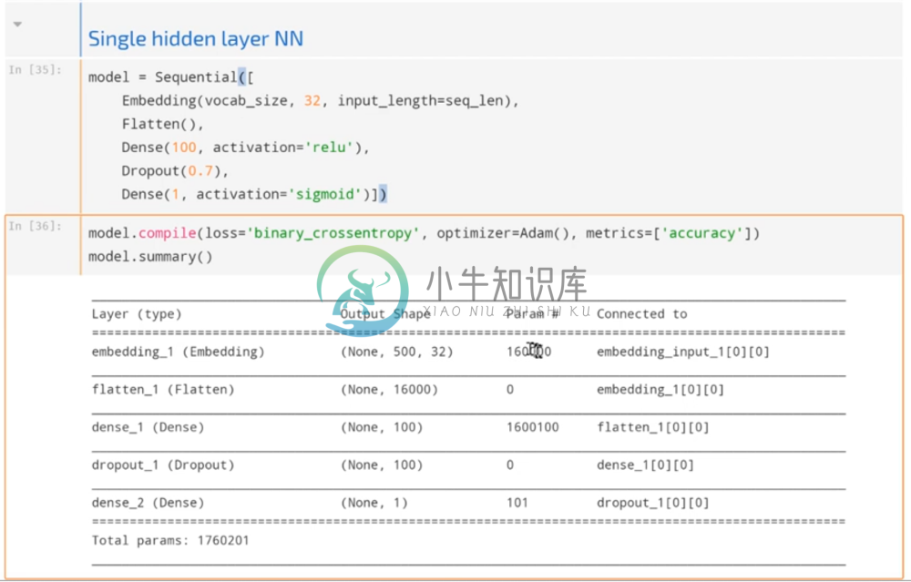
To start, we’ll use a simple Single Hidden Layer architecture.

Note that the first thing we start with is an embedding! The purpose of using these word id’s is to give each word a specific embedding, and then we can train the parameters in these embeddings to optimize for our desired task. In our case, we use 32 elements per embedding. We then flatten these elements out, and pass the entire vector to the rest of our standard architecture as usual. In our example, this simple neural network produced competitive results when compared to academia.

It’s important to note the information that is being captured here. For each review, we take a 500-element vector, look up the embeddings for each index, and return a flattened vector of length 500*32 and then pass this to a weight matrix. Therefore, the first 32 elements of this flattened vector are the embedding elements of the first word, the next 32 elements are the embedding of the second word, and so on and so forth. Thus not only does our model take into consideration the individual latent factors for each word, but it also cares about the position of that word in the review, since the columns of the fully connected weight matrix directly correspond to position.

CNN model 00:56:00

Of course, a better approach is to simply use a convolutional neural network. Hopefully you understand by now that convolutional neural networks are important whenever ordering in your data is important, which is clearly the case when dealing with a sentence.

Unlike our previous CNN’s for image recognition, this model uses 1-dimensional convolutions since our sentence is one-dimensional. Here, we apply 64 filters that cover five consecutive words at a time. We then apply max pooling and dropout as usual, and pass to fully-connected layers.

This simple convolutional neural network gives us a result of 89.47% validation accuracy, which beats the academic state-of-the-art.

Aside on 1-Dimensional Convolutions

It’s important to point out what we mean when we say 1-dimensional convolution. The filters in this case act on five words at a time; each word itself is a vector of 32 elements. Therefore the filter is itself a 5x32 matrix that dot products with the 5x32 matrix that represents the sequence of 5 words. If the filter is still 2 dimensional, what exactly do we mean by 1-dimensional convolution? What we mean is the propagation of the filter across the input matrix. In this example, the 5x32 filter slides across each consecutive five words represented in the matrix, and this can be visualized as the filter simply sliding down the matrix. In other words, the filter moves in one. direction. Contrast this with a 2-dimensional convolution, which slides not only across the rows but across the columns as well.

For more information on understanding convolutions, this article is very helpful.

Pre-Trained Word Embedding 01:12:00

Similar to our collaborative filtering example, the embeddings for each word are latent factors created by gradient descent that encapsulates information about the word. Specifically, when we start with randomly initialized embeddings, we train said embeddings to provide information about each word that is relevant to a specific task.

We might guess, and correctly so, that we can save a lot of time and effort by starting with pre-trained embeddings and fine-tuning them to suit our task. This makes sense because while we would expect the embeddings to differ depending on what the task is, we wouldn’t expect it to differ that much.

This is very similar to using a pre-trained network like VGG for image classification, and fine-tuning it to accomplish a different yet similar task. These are both examples of what is known as transfer learning.

Fortunately, pre-trained word embeddings are remarkably easy to utilize, since there is only ever one representation of a word. In comparison, consider the weights trained on Imagenet, and specifically the weights and filters that are useful in identifying images of dogs. These weights have been trained to perform well on Imagenet’s pictures of dogs, but they may not perform well on a different set of dog images that vary drastically from the dog images in Imagenet. With word embeddings however, there is only one representation of the word dog and it’s “dog”. Therefore we don’t have to worry about whether pre-trained embeddings will work well with our words because they are represented in the exact same way.

Two popular pre-trained word embeddings are:

• Glove: GloVe: Global Vectors for Word Representation
• Word2Vec: Paper

We’ll be using the GloVe embeddings. There are a variety of different embeddings available that have been trained on different corpuses, including Wikipedia, a massive database of newspaper articles, and a text dump of the entire internet. Some embeddings are cased and some are not, and there are small and large size embeddings for the level of complexity you desire.

From now on, we should always use pre-trained word embeddings anytime we do NLP. As we might expect, if we initialize our embeddings with pre-trained ones in our simple CNN from earlier, we get better results without even training them. Of course, allowing them to be trained allows us to finetune the embeddings for our purposes and this achieves the best result.

Unsupervised Learning for Word Embeddings

Given that we’ve previously constructed our word embeddings through optimizing a certain task such as classification, it’s reasonable to wonder what exactly these massive unlabeled text dumps were trained on. Since these are unlabelled, this is an example of unsupervised learning, and the goal here is to design some task that reveals information about the structure of these embeddings inherent in the data itself.

In the case of Word2Vec, the idea was to create a classification problem from the data itself. For example, we could take a sequence of 11 words, and then make a copy of it where the middle word is replaced with a random word. Most likely, this copy with a random word in the middle makes no sense, while the original does. Therefore, we can create a classification task by labeling the original sequence of eleven words as correct (1), and the random word copy as incorrect (0), and we can do this for every sequence of 11 words in the entire corpus. Finally, we can train on both the original and random word copies to learn embeddings. Again, this works because we’re extremely confident that a sentence with a random word inserted in the middle makes no sense, and therefore we’re certain that overwhelmingly our constructed labels will be correct.

Of course, this particularly task isn’t particularly useful, but in solving it on such a massive dataset these embeddings provide us with fairly general embeddings that aren’t specific to a particular task. This makes sense because the task itself involves simply understanding words and their contexts, and when a word is inappropriate or doesn’t make sense.

You can find more information on Word2Vec embeddings here

Visualizing Word Embeddings

We’ll use GloVe’s embeddings trained from Wikipedia, which is uncased and has 6 billion tokens. The 50 dimensional embeddings should be good for our purposes.

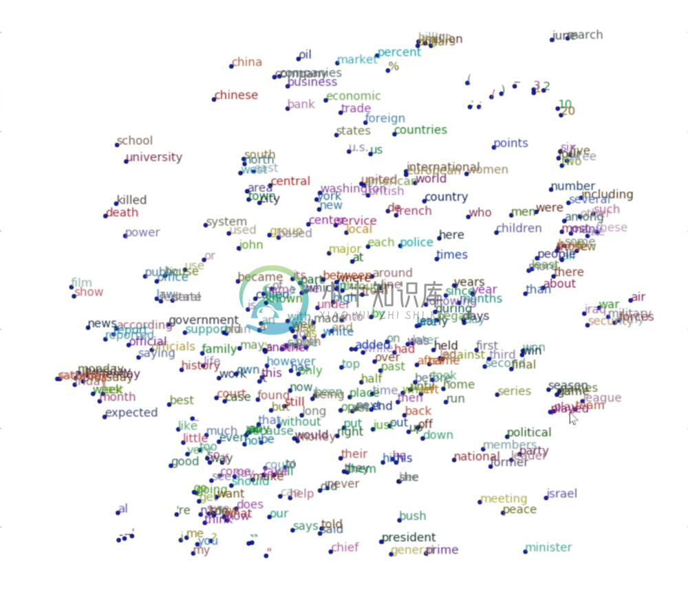
Like we did with our movie embeddings, we can use visualization techniques to see how effective these embeddings are at capturing information about these words. We will use T-sne, which is a dimensionality reduction algorithm to reduce the dimensions and allow us to visualize our words. It transforms our 50 dimensions into 2, while trying to keep those vectors that were close in 50 dimensions close in 2 dimensions.

We can see that many words we’d expect to be close together are indeed close. For example, school and university, killed and death, and even punctuations are grouped together. Of course there is some loss of information in these projections; notice the placement of bush next to president and general. We might expect a projection to show bush next to other plants, however this projection chose to place it near president and general because of President George W. Bush. In projecting, we’ve lost that additional information that we know should be present in the complete embedding, and we might expect that a different projection would place bush next to tree.

Using Glove for sentiment analysis:

Multi-Size CNN’s

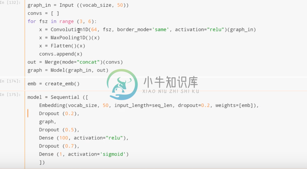
Before we move on to a brand new architecture, we wanted to mention a CNN variant that is worth taking a look at. Typically when tuning convolutional filter sizes, we settle on the optimal filter size. However, we could also simply build a model that performs convolutions with a range of different filter sizes, and then concatenates the outputs before continuing through dense layers.

Below is an implementation of this idea in Keras using the functional API to create the multiple convolution layer, and combining it with standard architecture using the sequential API.

Indeed, this architecture boosted our performance in the iMBD Sentiment dataset from our previous best result, to about 90.36%.

Recurrent Neural Network (RNN)

We conclude this lesson with a brief introduction to Recurrent Neural Networks.

The Need for RNN’s

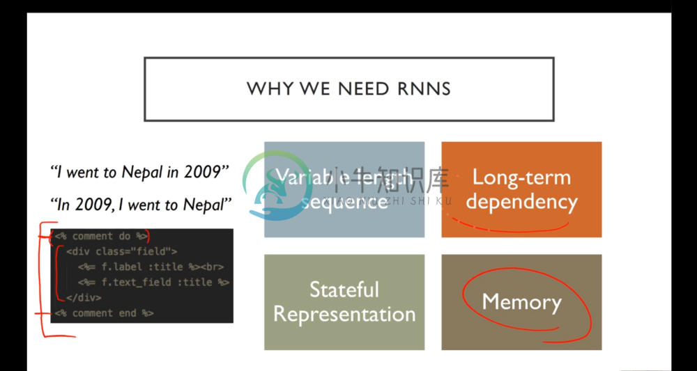
CNN’s have done a great job with the tasks we’ve discussed so far. However, let’s consider the following task:

How would we go about modeling the markup on the left? In other words, how do we build a model that understands the rules and conventions of predicting output that follows the conventions of the data it’s trained upon?

In the example of this XML-like markup, our model needs to remember things like closing XML tags after one has been opened. Specifically, the model has to keep memory about what has happened in the past in order to do so. This memory serves to keep track of long-term dependencies between things like opening and closing tags.

Consider also a model that is able to understand that the two sentences on the left mean the same thing. In order to do this, we need to keep track of state. This means that once we read that you’re in Nepal, and then read that it’s 2009, you know that this means “in Nepal in 2009”, and therefore when you read the same statement in the opposite order, you arrive at an equivalent outcome. This can be accomplished through stateful representation, which can remember previous things that happened in order to arrive at a complete picture of the event.

Finally, we would like a model that can handle variable length sequences. This is useful in dealing with data that has many different kinds of structures.

Convolutional neural networks don’t do this well, but Recurrent neural networks do.

Here is a great blog post on RNNs: The Unreasonable Effectiveness of Recurrent Neural Networks. In it we can see a recurrent neural network actively figuring out what the next state should be to effectively capture the necessary information in a Google Street View image to get an address.

Thinking about Neural Networks as Computational Graphs

Before we get to the fine details on RNN’s next lesson, we find it helpful to understand neural networks as computational graphs.

Below is a basic single hidden layer NN, represented as a computational graph.

In this representation, each shape represents a matrix, and each arrow represents some action on that matrix. Here, we have the input matrix represented by the rectangle at the bottom, and the first arrow symbolizes the matrix product with the first weight matrix followed by a rectified linear unit as an activation. The output of this first step (the hidden layer) is symbolized by the circle, which then undergoes a second and final weight matrix product, followed by a softmax function. This produces our output prediction matrix, as represented by the triangle.

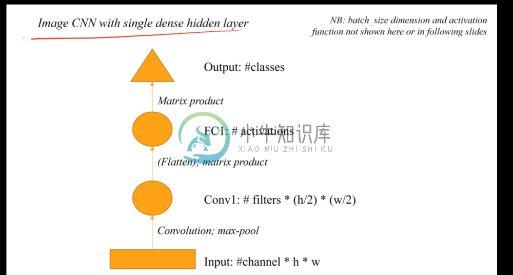
Next let’s look at a computational graph for a CNN.

This representation is self-explanatory.

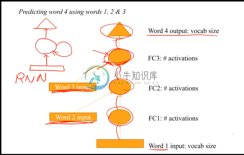
Now let’s look at the following graph.

The purpose of the architecture here is to predict what the next word will be, given the previous three words and their order.

Here, we take the word 1 input and put it through two layer transformations. After the second transformation, we merge it with the word 2 input, which itself has also been transformed. The meeting of the two arrows indicates a merge, and we’ll define it as either a sum of the two activations or a concatenation. We then perform a layer transformation on this merged matrix, and merge with a transformation of the word 3 input. Finally, we transform this last merged matrix into the output.

How is this different than building a model that takes as input all three words and combines them? The difference lies in the property of state. When we merge the second word input to the model, we’re merging a transformation of it after the model has transformed the first word twice. Therefore, the second layer (second circle) represents not only information from the word 2 input, but information about the word that came before it. The same applies for the merging of the third word. This is different than separately combining models because this architecture forces the information from word 2 to depend on word 1, and information from word 3 to depend on word 1 and 2. Thus, the network will learn what it needs to know from the first word to successfully make a prediction with the second word once they’ve been merged, and the same for the third word.

We can build such architectures for predicting words after any length of sequences. However, there is a much more flexible architecture that allows us to do this for sequential word prediction at any length. The key is to simply use a recurring layer, and this is what is known as a Recurrent Neural Network.

The top-left corner of the above image shows the basic idea. A word is given as an input, and goes through a layer transformation. Once transformed, it goes through a second transformation to output the predicted word. However, it also goes through a third transformation; this third transformation is indicated by the arrow pointing at itself, and what it does is transforms the hidden layer, and then merges it with the untransformed hidden layer. The weight matrix indicated by this arrow not only captures information about what word this hidden layer is going to predict, it also knows how to transform this information in an optimal way for merging with the previous hidden layer.

Now, the hidden layer consists not only of information about the second word, but since it was merged with the hidden layer before it, it contains state about the word prior to it. This builds ad infinitum, allowing RNN’s to keep track of all the states prior to the current word, and making the best prediction for what the next word should be.

RNN example code for words prediction

We briefly see how to use keras LSTM layer for predicting following words given a sentence.

• Train on random text. IP = 40 charachter sequence, OP= char at 40+1
• Generate 320 chars prediction with a seed text.
• Performs better for every iteration

Next lesson, we will continue to dive deeper into RNN’s and their uses.

This week’s links

• The lesson video

• The lesson 5 notes (includes time lines)

• The notebooks:

  • Lesson 5 shows the IMDB sentiment analysis
  • Word vectors contains the visualization of glove vectors
  • char-rnn is the RNN “Nietzsche generator” - we only briefly looked at this; we’ll be discussing this notebook more next week
  • Imagenet batchnorm is the method used to add batchnorm to imagenet. This is optional - now that we’ve done this for you, it’s included in vgg16bn.py; we’re providing the notebook for those of you that are interesting in learning how we did it

• The python scripts:

  • The VGG network with batchnorm - we will use this now instead of vgg16.py and automatically downloads the new weights when first used
  • utils.py - For finetuning, we will start using vgg_ft_bn (which uses VGG with batch norm) instead of vgg_ft

• The datasets:

  • The IMDB dataset is part of keras, and download code is part of the lesson 5 notebook.

• Pre-trained networks:

  • GloVe: Global Vectors for Word Representation
  • Vector Representations of Words - TensorFlow (word2vec)
  • SyntaxNet: Neural Models of Syntax

Information about this week’s topics

• Ben’s excellent blog post describing how he used deep learning for NLP at his startup, Quid
• Learning Word Vectors for Sentiment Analysis - the Stanford paper introducing the IMDB sentiment dataset
• An introduction to Principal Component Analysis (PCA)
• Understanding Convolutions - Chris Olah’s blog
• Exploring the Limits of Language Modeling

Assignments

• Try to make sure you’ve completed the key goals from previous weeks - top 50% of kaggle result on each of:

  • dogs and cats redux
  • state farm

• if you’ve already done that, try to either:

  • beat my imdb sentiment result, or (better still)…
  • use your own text classification dataset - like @bowles did in https://quid.com/feed/how-quid-uses-deep-learning-with-small-data .