第 15 章 Cypher 查询语言

优质

小牛编辑

112浏览

2023-12-01

Cypheris a declarative graph query language that allows for expressive and efficient querying and updating of the graph store without having to write traversals through the graph structure in code. Cypher is still growing and maturing, and that means that there probably will be breaking syntax changes. It also means that it has not undergone the same rigorous performance testing as other Neo4j components.

Cypher is designed to be a humane query language, suitable for both developers and (importantly, we think) operations professionals who want to make ad-hoc queries on the database. Our guiding goal is to make the simple things simple, and the complex things possible. Its constructs are based on English prose and neat iconography, which helps to make it (somewhat) self-explanatory.

Cypher is inspired by a number of different approaches and builds upon established practices for expressive querying. Most of the keywords like WHEREand ORDER BYare inspired by SQL. Pattern matching borrows expression approaches from SPARQL.

Being a declarative language, Cypher focuses on the clarity of expressing whatto retrieve from a graph, not howto do it, in contrast to imperative languages like Java, and scripting languages like Gremlin(supported via the 第 18.18 节 “Gremlin Plugin”) and the JRuby Neo4j bindings. This makes the concern of how to optimize queries an implementation detail not exposed to the user.

The query language is comprised of several distinct clauses.

- START: Starting points in the graph, obtained via index lookups or by element IDs.

- MATCH: The graph pattern to match, bound to the starting points in START.

- WHERE: Filtering criteria.

- RETURN: What to return.

- CREATE: Creates nodes and relationships.

- DELETE: Removes nodes, relationships and properties.

- SET: Set values to properties.

- FOREACH: Performs updating actions once per element in a list.

- WITH: Divides a query into multiple, distinct parts.

Let’s see three of them in action.

Imagine an example graph like the following one:

图 15.1. Example Graph

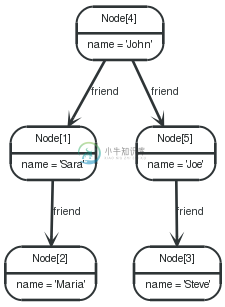
For example, here is a query which finds a user called John in an index and then traverses the graph looking for friends of Johns friends (though not his direct friends) before returning both John and any friends-of-friends that are found.

STARTjohn=node:node_auto_index(name = 'John')

MATCHjohn-[:friend]->()-[:friend]->fof

RETURNjohn, fof

Resulting in:

表 . --docbook

john	fof
2 rows
3 ms
Node[4]{name:"John"}	Node[2]{name:"Maria"}
Node[4]{name:"John"}	Node[3]{name:"Steve"}

Next up we will add filtering to set more parts in motion:

In this next example, we take a list of users (by node ID) and traverse the graph looking for those other users that have an outgoing friendrelationship, returning only those followed users who have a nameproperty starting with S.

STARTuser=node(5,4,1,2,3)

MATCHuser-[:friend]->follower

WHEREfollower.name =~ 'S.*'

RETURNuser, follower.name

Resulting in

表 . --docbook

user	follower.name
2 rows
1 ms
Node[5]{name:"Joe"}	"Steve"
Node[4]{name:"John"}	"Sara"

To use Cypher from Java, see 第 4.10 节 “在Java中执行Cypher查询”. For more Cypher examples, see 第 7 章数据模型范例as well.

15.1. 操作符

Operators in Cypher are of three different varieties — mathematical, equality and relationships.

The mathematical operators are +, -, *, /and %. Of these, only the plus-sign works on strings and collections.

The equality operators are =, <>, <, >, <=, >=.

Since Neo4j is a schema-free graph database, Cypher has two special operators — ?and !.

They are used on properties, and are used to deal with missing values. A comparison on a property that does not exist would normally cause an error. Instead of having to always check if the property exists before comparing its value with something else, the question mark make the comparison always return true if the property is missing, and the exclamation mark makes the comparator return false.

This predicate will evaluate to true if n.propis missing.

WHERE n.prop? = "foo"

This predicate will evaluate to false if n.propis missing.

WHERE n.prop! = "foo"

		警告
Mixing the two in the same comparison will lead to unpredictable results.

This is really syntactic sugar that expands to this:

WHERE n.prop? = "foo"⇒WHERE (not(has(n.prop)) OR n.prop = "foo")

WHERE n.prop! = "foo"⇒WHERE (has(n.prop) AND n.prop = "foo")

15.2. 表达式

15.2.1. Note on string literals

An expression in Cypher can be:

- A numeric literal (integer or double): 13, 40000, 3.14.

- A string literal: "Hello", 'World'.

- A boolean literal: true, false, TRUE, FALSE.

- An identifier: n, x, rel, myFancyIdentifier, `A name with weird stuff in it[]!`.

- A property: n.prop, x.prop, rel.thisProperty, myFancyIdentifier.`(weird property name)`.

- A nullable property: it’s a property, with a question mark or exclamation mark — n.prop?, rel.thisProperty!.

- A parameter: {param}, {0}

- A collection of expressions: ["a", "b"], [1,2,3], ["a", 2, n.property, {param}], [ ].

- A function call: length(p), nodes(p).

- An aggregate function: avg(x.prop), count(*).

- Relationship types: :REL_TYPE, :`REL TYPE`, :REL1|REL2.

- A path-pattern: a-->()<--b.

15.2.1. Note on string literals

String literals can contain these escape sequences.

Escape sequence	Character
\t	Tab
\b	Backspace
\n	Newline
\r	Carriage return
\f	Form feed
\'	Single quote
\"	Double quote
\\	Backslash

15.3. 参数

Cypher supports querying with parameters. This allows developers to not to have to do string building to create a query, and it also makes caching of execution plans much easier for Cypher.

Parameters can be used for literals and expressions in the WHEREclause, for the index key and index value in the STARTclause, index queries, and finally for node/relationship ids. Parameters can not be used as for property names, since property notation is part of query structure that is compiled into a query plan.

Accepted names for parameter are letters and number, and any combination of these.

Here follows a few examples of how you can use parameters from Java.

Parameter for node id.

Map<String, Object> params = newHashMap<String, Object>();

params.put( "id", 0);

ExecutionResult result = engine.execute( "start n=node({id}) return n.name", params );

Parameter for node object.

Map<String, Object> params = newHashMap<String, Object>();

params.put( "node", andreasNode );

ExecutionResult result = engine.execute( "start n=node({node}) return n.name", params );

Parameter for multiple node ids.

Map<String, Object> params = newHashMap<String, Object>();

params.put( "id", Arrays.asList( 0, 1, 2) );

ExecutionResult result = engine.execute( "start n=node({id}) return n.name", params );

Parameter for string literal.

Map<String, Object> params = newHashMap<String, Object>();

params.put( "name", "Johan");

ExecutionResult result =

engine.execute( "start n=node(0,1,2) where n.name = {name} return n", params );

Parameter for index key and value.

Map<String, Object> params = newHashMap<String, Object>();

params.put( "key", "name");

params.put( "value", "Michaela");

ExecutionResult result =

engine.execute( "start n=node:people({key} = {value}) return n", params );

Parameter for index query.

Map<String, Object> params = newHashMap<String, Object>();

params.put( "query", "name:Andreas");

ExecutionResult result = engine.execute( "start n=node:people({query}) return n", params );

Numeric parameters for SKIPand LIMIT.

Map<String, Object> params = newHashMap<String, Object>();

params.put( "s", 1);

params.put( "l", 1);

ExecutionResult result =

engine.execute( "start n=node(0,1,2) return n.name skip {s} limit {l}", params );

Parameter for regular expression.

Map<String, Object> params = newHashMap<String, Object>();

params.put( "regex", ".*h.*");

ExecutionResult result =

engine.execute( "start n=node(0,1,2) where n.name =~ {regex} return n.name", params );

15.4. 标识符

When you reference parts of the pattern, you do so by naming them. The names you give the different parts are called identifiers.

In this example:

1	STARTn=node(1) MATCHn-->b RETURNb

The identifiers are nand b.

Identifier names are case sensitive, and can contain underscores and alphanumeric characters (a-z, 0-9), but must start with a letter. If other characters are needed, you can quote the identifier using backquote (`) signs.

The same rules apply to property names.

15.5. 备注

To add comments to your queries, use double slash. Examples:

STARTn=node(1) RETURNb //This is an end of line comment

STARTn=node(1)

//This is a whole line comment

RETURNb

1	STARTn=node(1) WHEREn.property = "//This is NOT a comment"RETURNb

15.6. 更新图数据库

15.6.1. The Structure of Updating Queries

15.6.2. Returning data

Cypher can be used for both querying and updating your graph.

15.6.1. The Structure of Updating Queries

Quick info

- A Cypher query part can’t both match and update the graph at the same time.

- Every part can either read and match on the graph, or make updates on it.

If you read from the graph, and then update the graph, your query implicitly has two parts — the reading is the first part, and the writing is the second. If your query is read-only, Cypher will be lazy, and not actually pattern match until you ask for the results. Here, the semantics are that allthe reading will be done before any writing actually happens. This is very important — without this it’s easy to find cases where the pattern matcher runs into data that is being created by the very same query, and all bets are off. That road leads to Heisenbugs, Brownian motion and cats that are dead and alive at the same time.

First reading, and then writing, is the only pattern where the query parts are implicit — any other order and you have to be explicit about your query parts. The parts are separated using the WITHstatement. WITHis like the event horizon — it’s a barrier between a plan and the finished execution of that plan.

When you want to filter using aggregated data, you have to chain together two reading query parts — the first one does the aggregating, and the second query filters on the results coming from the first one.

STARTn=node(...)

MATCHn-[:friend]-friend

WITHn, count(friend) asfriendsCount

WHEREfriendsCount > 3

RETURNn, friendsCount

Using WITH, you specify how you want the aggregation to happen, and that the aggregation has to be finished before Cypher can start filtering.

You can chain together as many query parts as you have JVM heap for.

15.6.2. Returning data

Any query can return data. If your query only reads, it has to return data — it serves no purpose if it doesn’t, and it is not a valid Cypher query. Queries that update the graph don’t have to return anything, but they can.

After all the parts of the query comes one final RETURNstatement. RETURNis not part of any query part — it is a period symbol after an eloquent statement. When RETURNis legal, it’s also legal to use SKIP/LIMITand ORDER BY.

If you return graph elements from a query that has just deleted them — beware, you are holding a pointer that is no longer valid. Operations on that node might fail mysteriously and unpredictably.

15.7. 事务

Any query that updates the graph will run in a transaction. An updating query will always either fully succeed, or not succeed at all.

Cypher will either create a new transaction, and commit it once the query finishes. Or if a transaction already exists in the running context, the query will run inside it, and nothing will be persisted to disk until the transaction is successfully committed.

This can be used to have multiple queries be committed as a single transaction:

1.Open a transaction,

2.run multiple updating Cypher queries,

3.and commit all of them in one go.

Note that a query will hold the changes in heap until the whole query has finished executing. A large query will consequently need a JVM with lots of heap space.

15.8. Patterns

Patterns are at the very core of Cypher, and are used in a lot of different places. Using patterns, you describe the shape of the data that you are looking for. Patterns are used in the MATCHclause. Path patterns are expressions. Since these expressions are collections, they can also be used as predicates (a non-empty collection signifies true). They are also used to CREATE/CREATE UNIQUEthe graph.

So, understanding patterns is important, to be able to be effective with Cypher.

You describe the pattern, and Cypher will figure out how to get that data for you. The idea is for you to draw your query on a whiteboard, naming the interesting parts of the pattern, so you can then use values from these parts to create the result set you are looking for.

Patterns have bound points, or starting points. They are the parts of the pattern that are already “bound” to a set of graph nodes or relationships. All parts of the pattern must be directly or indirectly connected to a starting point — a pattern where parts of the pattern are not reachable from any starting point will be rejected.

Clause	Optional	Multiple rel. types	Varlength	Paths	Maps
Match	Yes	Yes	Yes	Yes	-
Create	-	-	-	Yes	Yes
Create Unique	-	-	-	Yes	Yes
Expressions	-	Yes	Yes	-	-

15.8.1. Patterns for related nodes

The description of the pattern is made up of one or more paths, separated by commas. A path is a sequence of nodes and relationships that always start and end in nodes. An example path would be:

(a)-->(b)

This is a path starting from the pattern node a, with an outgoing relationship from it to pattern node b.

Paths can be of arbitrary length, and the same node may appear in multiple places in the path.

Node identifiers can be used with or without surrounding parenthesis. The following match is semantically identical to the one we saw above — the difference is purely aesthetic.

a-->b

If you don’t care about a node, you don’t need to name it. Empty parenthesis are used for these nodes, like so:

a-->()<--b

15.8.2. Working with relationships

If you need to work with the relationship between two nodes, you can name it.

a-[r]->b

If you don’t care about the direction of the relationship, you can omit the arrow at either end of the relationship, like this:

a--b

Relationships have types. When you are only interested in a specific relationship type, you can specify this like so:

a-[:REL_TYPE]->b

If multiple relationship types are acceptable, you can list them, separating them with the pipe symbol |like this:

a-[r:TYPE1|TYPE2]->b

This pattern matches a relationship of type TYPE1or TYPE2, going from ato b. The relationship is named r. Multiple relationship types can not be used with CREATEor CREATE UNIQUE.

15.8.3. Optional relationships

An optional relationship is matched when it is found, but replaced by a nullotherwise. Normally, if no matching relationship is found, that sub-graph is not matched. Optional relationships could be called the Cypher equivalent of the outer join in SQL.

They can only be used in MATCH.

Optional relationships are marked with a question mark. They allow you to write queries like this one:

Query

STARTme=node(*)

MATCHme-->friend-[?]->friend_of_friend

RETURNfriend, friend_of_friend

The query above says “for every person, give me all their friends, and their friends friends, if they have any.”

Optionality is transitive — if a part of the pattern can only be reached from a bound point through an optional relationship, that part is also optional. In the pattern above, the only bound point in the pattern is me. Since the relationship between friendand childrenis optional, childrenis an optional part of the graph.

Also, named paths that contain optional parts are also optional — if any part of the path is null, the whole path is null.

In the following examples, band pare all optional and can contain null:

Query

STARTa=node(4)

MATCHp = a-[?]->b

RETURNb

Query

STARTa=node(4)

MATCHp = a-[?*]->b

RETURNb

Query

STARTa=node(4)

MATCHp = a-[?]->x-->b

RETURNb

Query

STARTa=node(4), x=node(3)

MATCHp = shortestPath( a-[?*]->x )

RETURNp

15.8.4. Controlling depth

A pattern relationship can span multiple graph relationships. These are called variable length relationships, and are marked as such using an asterisk (*):

(a)-[*]->(b)

This signifies a path starting on the pattern node a, following only outgoing relationships, until it reaches pattern node b. Any number of relationships can be followed searching for a path to b, so this can be a very expensive query, depending on what your graph looks like.

You can set a minimum set of steps that can be taken, and/or the maximum number of steps:

(a)-[*3..5]->(b)

This is a variable length relationship containing at least three graph relationships, and at most five.

Variable length relationships can not be used with CREATEand CREATE UNIQUE.

As a simple example, let’s take the query below:

Query

STARTme=node(3)

MATCHme-[:KNOWS*1..2]-remote_friend

RETURNremote_friend

表 . --docbook

remote_friend

2 rows

0 ms

Node[1]{name:"Dilshad"}

Node[4]{name:"Anders"}

This query starts from one node, and follows KNOWSrelationships two or three steps out, and then stops.

15.8.5. Assigning to path identifiers

In a graph database, a path is a very important concept. A path is a collection of nodes and relationships, that describe a path in the graph. To assign a path to a path identifier, you simply assign a path pattern to an identifier, like so:

p = (a)-[*3..5]->(b)

You can do this in MATCH, CREATEand CREATE UNIQUE, but not when using patterns as expressions. Example of the three in a single query:

Query

STARTme=node(3)

MATCHp1 = me-[*2]-friendOfFriend

CREATEp2 = me-[:MARRIED_TO]-(wife {name:"Gunhild"})

CREATEUNIQUEp3 = wife-[:KNOWS]-friendOfFriend

RETURNp1,p2,p3

15.8.6. Setting properties

Nodes and relationships are important, but Neo4j uses properties on both of these to allow for far denser graphs models.

Properties are expressed in patterns using the map-construct, which is simply curly brackets surrounding a number of key-expression pairs, separated by commas, e.g. { name: "Andres", sport: "BJJ" }. If the map is supplied through a parameter, the normal parameter expression is used: { paramName }.

Maps are only used by CREATEand CREATE UNIQUE. In CREATEthey are used to set the properties on the newly created nodes and relationships.

When used with CREATE UNIQUE, they are used to try to match a pattern element with the corresponding graph element. The match is successful if the properties on the pattern element can be matched exactly against properties on the graph elements. The graph element can have additional properties, and they do not affect the match. If Neo4j fails to find matching graph elements, the maps is used to set the properties on the newly created elements.

15.8.7. Start

Every query describes a pattern, and in that pattern one can have multiple starting points. A starting point is a relationship or a node where a pattern is anchored. You can either introduce starting points by id, or by index lookups. Note that trying to use an index that doesn’t exist will throw an exception.

Graph

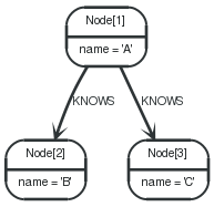
Node by id

Binding a node as a starting point is done with the node(*)function .

Query

1 2	STARTn=node(1) RETURNn

The corresponding node is returned.

表 . --docbook

1 row

0 ms

Node[1]{name:"A"}

Relationship by id

Binding a relationship as a starting point is done with the relationship(*)function, which can also be abbreviated rel(*).

Query

1 2	STARTr=relationship(0) RETURNr

The relationship with id 0is returned.

表 . --docbook

1 row

0 ms

:KNOWS[0] {}

Multiple nodes by id

Multiple nodes are selected by listing them separated by commas.

Query

1 2	STARTn=node(1, 2, 3) RETURNn

This returns the nodes listed in the STARTstatement.

表 . --docbook

3 rows

0 ms

Node[1]{name:"A"}

Node[2]{name:"B"}

Node[3]{name:"C"}

All nodes

To get all the nodes, use an asterisk. This can be done with relationships as well.

Query

1 2	STARTn=node(*) RETURNn

This query returns all the nodes in the graph.

表 . --docbook

3 rows

0 ms

Node[1]{name:"A"}

Node[2]{name:"B"}

Node[3]{name:"C"}

Node by index lookup

When the starting point can be found by using index lookups, it can be done like this: node:index-name(key = "value"). In this example, there exists a node index named nodes.

Query

1 2	STARTn=node:nodes(name = "A") RETURNn

The query returns the node indexed with the name "A".

表 . --docbook

1 row

0 ms

Node[1]{name:"A"}

Relationship by index lookup

When the starting point can be found by using index lookups, it can be done like this: relationship:index-name(key = "value").

Query

1 2	STARTr=relationship:rels(name = "Andrés") RETURNr

The relationship indexed with the nameproperty set to "Andrés" is returned by the query.

表 . --docbook

1 row

0 ms

:KNOWS[0] {name:"Andrés"

Node by index query

When the starting point can be found by more complex Lucene queries, this is the syntax to use: node:index-name("query").This allows you to write more advanced index queries.

Query

1 2	STARTn=node:nodes("name:A") RETURNn

The node indexed with name "A" is returned by the query.

表 . --docbook

1 row

0 ms

Node[1]{name:"A"}

Multiple starting points

Sometimes you want to bind multiple starting points. Just list them separated by commas.

Query

1 2	STARTa=node(1), b=node(2) RETURNa,b

Both the nodes Aand the Bare returned.

表 . --docbook

a	b
1 row
0 ms
Node[1]{name:"A"}	Node[2]{name:"B"}

15.8.8. Match

Introduction

		提示
In the MATCHclause, patterns are used a lot. Read 第 15.8 节 “Patterns”for an introduction.

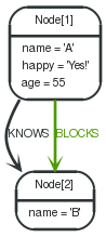
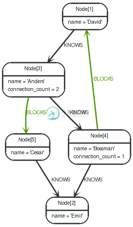
The following graph is used for the examples below:

Graph

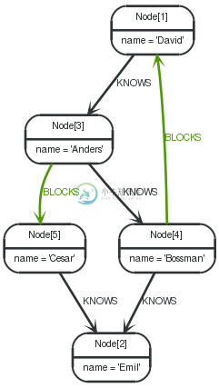
Related nodes

The symbol --means related to,without regard to type or direction.

Query

STARTn=node(3)

MATCH(n)--(x)

RETURNx

All nodes related to A (Anders) are returned by the query.

表 . --docbook

3 rows

0 ms

Node[4]{name:"Bossman"}

Node[1]{name:"David"}

Node[5]{name:"Cesar"}

Outgoing relationships

When the direction of a relationship is interesting, it is shown by using -->or <--, like this:

Query

STARTn=node(3)

MATCH(n)-->(x)

RETURNx

All nodes that A has outgoing relationships to are returned.

表 . --docbook

2 rows

0 ms

Node[4]{name:"Bossman"}

Node[5]{name:"Cesar"}

Directed relationships and identifier

If an identifier is needed, either for filtering on properties of the relationship, or to return the relationship, this is how you introduce the identifier.

Query

STARTn=node(3)

MATCH(n)-[r]->()

RETURNr

The query returns all outgoing relationships from node A.

表 . --docbook

2 rows

0 ms

:KNOWS[0] {}

:BLOCKS[1] {}

Match by relationship type

When you know the relationship type you want to match on, you can specify it by using a colon together with the relationship type.

Query

STARTn=node(3)

MATCH(n)-[:BLOCKS]->(x)

RETURNx

All nodes that are BLOCKed by A are returned by this query.

表 . --docbook

1 row

0 ms

Node[5]{name:"Cesar"}

Match by multiple relationship types

To match on one of multiple types, you can specify this by chaining them together with the pipe symbol |.

Query

STARTn=node(3)

MATCH(n)-[:BLOCKS|KNOWS]->(x)

RETURNx

All nodes with a BLOCKor KNOWSrelationship to A are returned.

表 . --docbook

2 rows

0 ms

Node[5]{name:"Cesar"}

Node[4]{name:"Bossman"}

Match by relationship type and use an identifier

If you both want to introduce an identifier to hold the relationship, and specify the relationship type you want, just add them both, like this.

Query

STARTn=node(3)

MATCH(n)-[r:BLOCKS]->()

RETURNr

All BLOCKSrelationships going out from A are returned.

表 . --docbook

1 row

0 ms

:BLOCKS[1] {}

Relationship types with uncommon characters

Sometime your database will have types with non-letter characters, or with spaces in them. Use `(backtick) to quote these.

Query

STARTn=node(3)

MATCH(n)-[r:`TYPETHAT HASSPACE INIT`]->()

RETURNr

This query returns a relationship of a type with spaces in it.

表 . --docbook

1 row

0 ms

:TYPE THAT HAS SPACE IN IT[6] {}

Multiple relationships

Relationships can be expressed by using multiple statements in the form of ()--(), or they can be strung together, like this:

Query

STARTa=node(3)

MATCH(a)-[:KNOWS]->(b)-[:KNOWS]->(c)

RETURNa,b,c

The three nodes in the path are returned by the query.

表 . --docbook

a	b	c
1 row
0 ms
Node[3]{name:"Anders"}	Node[4]{name:"Bossman"}	Node[2]{name:"Emil"}

Variable length relationships

Nodes that are a variable number of relationship→node hops away can be found using the following syntax: -[:TYPE*minHops..maxHops]->. minHops and maxHops are optional and default to 1 and infinity respectively. When no bounds are given the dots may be omitted.

Query

STARTa=node(3), x=node(2, 4)

MATCHa-[:KNOWS*1..3]->x

RETURNa,x

This query returns the start and end point, if there is a path between 1 and 3 relationships away.

表 . --docbook

a	x
2 rows
0 ms
Node[3]{name:"Anders"}	Node[2]{name:"Emil"}
Node[3]{name:"Anders"}	Node[4]{name:"Bossman"}

Relationship identifier in variable length relationships

When the connection between two nodes is of variable length, a relationship identifier becomes an collection of relationships.

Query

STARTa=node(3), x=node(2, 4)

MATCHa-[r:KNOWS*1..3]->x

RETURNr

The query returns the relationships, if there is a path between 1 and 3 relationships away.

表 . --docbook

2 rows

0 ms

[:KNOWS[0] {},:KNOWS[3] {}]

[:KNOWS[0] {}]

Zero length paths

Using variable length paths that have the lower bound zero means that two identifiers can point to the same node. If the distance between two nodes is zero, they are by definition the same node.

Query

STARTa=node(3)

MATCHp1=a-[:KNOWS*0..1]->b, p2=b-[:BLOCKS*0..1]->c

RETURNa,b,c, length(p1), length(p2)

This query will return four paths, some of which have length zero.

表 . --docbook

a	b	c	length(p1)	length(p2)
4 rows
0 ms
Node[3]{name:"Anders"}	Node[3]{name:"Anders"}	Node[3]{name:"Anders"}	0	0
Node[3]{name:"Anders"}	Node[3]{name:"Anders"}	Node[5]{name:"Cesar"}	0	1
Node[3]{name:"Anders"}	Node[4]{name:"Bossman"}	Node[4]{name:"Bossman"}	1	0
Node[3]{name:"Anders"}	Node[4]{name:"Bossman"}	Node[1]{name:"David"}	1	1

Optional relationship

If a relationship is optional, it can be marked with a question mark. This is similar to how a SQL outer join works. If the relationship is there, it is returned. If it’s not, nullis returned in it’s place. Remember that anything hanging off an optional relationship, is in turn optional, unless it is connected with a bound node through some other path.

Query

STARTa=node(2)

MATCHa-[?]->x

RETURNa,x

A node, and nullare returned, since the node has no outgoing relationships.

表 . --docbook

a	x
1 row
0 ms
Node[2]{name:"Emil"}	<null>

Optional typed and named relationship

Just as with a normal relationship, you can decide which identifier it goes into, and what relationship type you need.

Query

STARTa=node(3)

MATCHa-[r?:LOVES]->()

RETURNa,r

This returns a node, and null, since the node has no outgoing LOVESrelationships.

表 . --docbook

a	r
1 row
0 ms
Node[3]{name:"Anders"}	<null>

Properties on optional elements

Returning a property from an optional element that is nullwill also return null.

Query

STARTa=node(2)

MATCHa-[?]->x

RETURNx, x.name

This returns the element x (nullin this query), and nullas it’s name.

表 . --docbook

x	x.name
1 row
0 ms
<null>	<null>

Complex matching

Using Cypher, you can also express more complex patterns to match on, like a diamond shape pattern.

Query

STARTa=node(3)

MATCH(a)-[:KNOWS]->(b)-[:KNOWS]->(c), (a)-[:BLOCKS]-(d)-[:KNOWS]-(c)

RETURNa,b,c,d

This returns the four nodes in the paths.

表 . --docbook

a	b	c	d
1 row
0 ms
Node[3]{name:"Anders"}	Node[4]{name:"Bossman"}	Node[2]{name:"Emil"}	Node[5]{name:"Cesar"}

Shortest path

Finding a single shortest path between two nodes is as easy as using the shortestPathfunction. It’s done like this:

Query

STARTd=node(1), e=node(2)

MATCHp = shortestPath( d-[*..15]->e )

RETURNp

This means: find a single shortest path between two nodes, as long as the path is max 15 relationships long. Inside of the parenthesis you define a single link of a path — the starting node, the connecting relationship and the end node. Characteristics describing the relationship like relationship type, max hops and direction are all used when finding the shortest path. You can also mark the path as optional.

表 . --docbook

1 row

0 ms

[Node[1]{name:"David"},:KNOWS[2] {},Node[3]{name:"Anders"},:KNOWS[0] {},Node[4]{name:"Bossman"},:KNOWS[3] {},Node[2]{name:"Emil"}]

All shortest paths

Finds all the shortest paths between two nodes.

Query

STARTd=node(1), e=node(2)

MATCHp = allShortestPaths( d-[*..15]->e )

RETURNp

This example will find the two directed paths between David and Emil.

表 . --docbook

2 rows

0 ms

[Node[1]{name:"David"},:KNOWS[2] {},Node[3]{name:"Anders"},:KNOWS[0] {},Node[4]{name:"Bossman"},:KNOWS[3] {},Node[2]{name:"Emil"}]

[Node[1]{name:"David"},:KNOWS[2] {},Node[3]{name:"Anders"},:BLOCKS[1] {},Node[5]{name:"Cesar"},:KNOWS[4] {},Node[2]{name:"Emil"}]

Named path

If you want to return or filter on a path in your pattern graph, you can a introduce a named path.

Query

STARTa=node(3)

MATCHp = a-->b

RETURNp

This returns the two paths starting from the first node.

表 . --docbook

2 rows

0 ms

[Node[3]{name:"Anders"},:KNOWS[0] {},Node[4]{name:"Bossman"}]

[Node[3]{name:"Anders"},:BLOCKS[1] {},Node[5]{name:"Cesar"}]

Matching on a bound relationship

When your pattern contains a bound relationship, and that relationship pattern doesn’t specify direction, Cypher will try to match the relationship where the connected nodes switch sides.

Query

STARTr=rel(0)

MATCHa-[r]-b

RETURNa,b

This returns the two connected nodes, once as the start node, and once as the end node.

表 . --docbook

a	b
2 rows
0 ms
Node[3]{name:"Anders"}	Node[4]{name:"Bossman"}
Node[4]{name:"Bossman"}	Node[3]{name:"Anders"}

Match with OR

Strictly speaking, you can’t do ORin your MATCH. It’s still possible to form a query that works a lot like OR.

Query

STARTa=node(3), b=node(2)

MATCHa-[?:KNOWS]-x-[?:KNOWS]-b

RETURNx

This query is saying: give me the nodes that are connected to a, or b, or both.

表 . --docbook

3 rows

0 ms

Node[4]{name:"Bossman"}

Node[5]{name:"Cesar"}

Node[1]{name:"David"}

15.8.9. Where

If you need filtering apart from the pattern of the data that you are looking for, you can add clauses in the WHEREpart of the query.

Graph

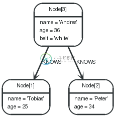
Boolean operations

You can use the expected boolean operators ANDand OR, and also the boolean function NOT().

Query

STARTn=node(3, 1)

WHERE(n.age < 30 andn.name = "Tobias") ornot(n.name = "Tobias")

RETURNn

This will return both nodes in the start clause.

表 . --docbook

2 rows

0 ms

Node[3]{name:"Andres",age:36,belt:"white"}

Node[1]{name:"Tobias",age:25}

Filter on node property

To filter on a property, write your clause after the WHEREkeyword. Filtering on relationship properties works just the same way.

Query

STARTn=node(3, 1)

WHEREn.age < 30

RETURNn

The "Tobias" node will be returned.

表 . --docbook

1 row

0 ms

Node[1]{name:"Tobias",age:25}

Regular expressions

You can match on regular expressions by using =~ "regexp", like this:

Query

STARTn=node(3, 1)

WHEREn.name =~ 'Tob.*'

RETURNn

The "Tobias" node will be returned.

表 . --docbook

1 row

0 ms

Node[1]{name:"Tobias",age:25}

Escaping in regular expressions

If you need a forward slash inside of your regular expression, escape it. Remember that back slash needs to be escaped in string literals

Query

STARTn=node(3, 1)

WHEREn.name =~ 'Some\\/thing'

RETURNn

No nodes match this regular expression.

表 . --docbook

0 row

0 ms

(empty result)

Case insensitive regular expressions

By pre-pending a regular expression with (?i), the whole expression becomes case insensitive.

Query

STARTn=node(3, 1)

WHEREn.name =~ '(?i)ANDR.*'

RETURNn

The node with name "Andres" is returned.

表 . --docbook

1 row

0 ms

Node[3]{name:"Andres",age:36,belt:"white"}

Filtering on relationship type

You can put the exact relationship type in the MATCHpattern, but sometimes you want to be able to do more advanced filtering on the type. You can use the special property TYPEto compare the type with something else. In this example, the query does a regular expression comparison with the name of the relationship type.

Query

STARTn=node(3)

MATCH(n)-[r]->()

WHEREtype(r) =~ 'K.*'

RETURNr

This returns relationships that has a type whose name starts with K.

表 . --docbook

2 rows

0 ms

:KNOWS[0] {}

:KNOWS[1] {}

Property exists

To only include nodes/relationships that have a property, use the HAS()function and just write out the identifier and the property you expect it to have.

Query

STARTn=node(3, 1)

WHEREhas(n.belt)

RETURNn

The node named "Andres" is returned.

表 . --docbook

1 row

0 ms

Node[3]{name:"Andres",age:36,belt:"white"}

Default true if property is missing

If you want to compare a property on a graph element, but only if it exists, use the nullable property syntax. You can use a question mark if you want missing property to return true, like:

Query

STARTn=node(3, 1)

WHEREn.belt? = 'white'

RETURNn

This returns all nodes, even those without the belt property.

表 . --docbook

2 rows

0 ms

Node[3]{name:"Andres",age:36,belt:"white"}

Node[1]{name:"Tobias",age:25}

Default false if property is missing

When you need missing property to evaluate to false, use the exclamation mark.

Query

STARTn=node(3, 1)

WHEREn.belt! = 'white'

RETURNn

No nodes without the belt property are returned.

表 . --docbook

1 row

0 ms

Node[3]{name:"Andres",age:36,belt:"white"}

Filter on null values

Sometimes you might want to test if a value or an identifier is null. This is done just like SQL does it, with IS NULL. Also like SQL, the negative is IS NOT NULL, although NOT(IS NULL x)also works.

Query

STARTa=node(1), b=node(3, 2)

MATCHa<-[r?]-b

WHEREr isnull

RETURNb

Nodes that Tobias is not connected to are returned.

表 . --docbook

1 row

0 ms

Node[2]{name:"Peter",age:34}

Filter on patterns

Patterns are expressions in Cypher, expressions that return a collection of paths. Collection expressions are also predicates — an empty collection represents false, and a non-empty represents true.

So, patterns are not only expressions, they are also predicates. The only limitation to your pattern is that you must be able to express it in a single path. You can not use commas between multiple paths like you do in MATCH. You can achieve the same effect by combining multiple patterns with AND.

Note that you can not introduce new identifiers here. Although it might look very similar to the MATCHpatterns, the WHEREclause is all about eliminating matched subgraphs. MATCH a-[*]->bis very different from WHERE a-[*]->b; the first will produce a subgraph for every path it can find between aand b, and the latter will eliminate any matched subgraphs where aand bdo not have a directed relationship chain between them.

Query

STARTtobias=node(1), others=node(3, 2)

WHEREtobias<--others

RETURNothers

Nodes that have an outgoing relationship to the "Tobias" node are returned.

表 . --docbook

others

1 row

0 ms

Node[3]{name:"Andres",age:36,belt:"white"}

Filter on patterns using NOT

The NOT()function can be used to exclude a pattern.

Query

STARTpersons=node(*), peter=node(2)

WHEREnot(persons-->peter)

RETURNpersons

Nodes that do not have an outgoing relationship to the "Peter" node are returned.

表 . --docbook

persons

2 rows

0 ms

Node[1]{name:"Tobias",age:25}

Node[2]{name:"Peter",age:34}

IN operator

To check if an element exists in a collection, you can use the INoperator.

Query

STARTa=node(3, 1, 2)

WHEREa.name IN["Peter", "Tobias"]

RETURNa

This query shows how to check if a property exists in a literal collection.

表 . --docbook

2 rows

0 ms

Node[1]{name:"Tobias",age:25}

Node[2]{name:"Peter",age:34}

15.8.10. Return

In the RETURNpart of your query, you define which parts of the pattern you are interested in. It can be nodes, relationships, or properties on these.

Graph

Return nodes

To return a node, list it in the RETURNstatemenet.

Query

1 2	STARTn=node(2) RETURNn

The example will return the node.

表 . --docbook

1 row

0 ms

Node[2]{name:"B"}

Return relationships

To return a relationship, just include it in the RETURNlist.

Query

STARTn=node(1)

MATCH(n)-[r:KNOWS]->(c)

RETURNr

The relationship is returned by the example.

表 . --docbook

1 row

0 ms

:KNOWS[0] {}

Return property

To return a property, use the dot separator, like this:

Query

1 2	STARTn=node(1) RETURNn.name

The value of the property namegets returned.

表 . --docbook

n.name

1 row

0 ms

"A"

Return all elements

When you want to return all nodes, relationships and paths found in a query, you can use the *symbol.

Query

STARTa=node(1)

MATCHp=a-[r]->b

RETURN*

This returns the two nodes, the relationship and the path used in the query.

表 . --docbook

a	b	r	p
2 rows
0 ms
Node[1]{name:"A",happy:"Yes!",age:55}	Node[2]{name:"B"}	:KNOWS[0] {}	[Node[1]{name:"A",happy:"Yes!",age:55},:KNOWS[0] {},Node[2]{name:"B"}]
Node[1]{name:"A",happy:"Yes!",age:55}	Node[2]{name:"B"}	:BLOCKS[1] {}	[Node[1]{name:"A",happy:"Yes!",age:55},:BLOCKS[1] {},Node[2]{name:"B"}]

Identifier with uncommon characters

To introduce a placeholder that is made up of characters that are outside of the english alphabet, you can use the `to enclose the identifier, like this:

Query

1 2	START`This isn't a common identifier`=node(1) RETURN `This isn't a common identifier`.happy

The node indexed with name "A" is returned

表 . --docbook

This isn't a common identifier.happy

1 row

0 ms

"Yes!"

Column alias

If the name of the column should be different from the expression used, you can rename it by using AS<new name>.

Query

1 2	STARTa=node(1) RETURNa.age ASSomethingTotallyDifferent

Returns the age property of a node, but renames the column.

表 . --docbook

SomethingTotallyDifferent

1 row

0 ms

Optional properties

If a property might or might not be there, you can select it optionally by adding a questionmark to the identifier, like this:

Query

1 2	STARTn=node(1, 2) RETURNn.age?

This example returns the age when the node has that property, or nullif the property is not there.

表 . --docbook

n.age?

2 rows

0 ms

<null>

Unique results

DISTINCTretrieves only unique rows depending on the columns that have been selected to output.

Query

STARTa=node(1)

MATCH(a)-->(b)

RETURNdistinctb

The node named B is returned by the query, but only once.

表 . --docbook

1 row

0 ms

Node[2]{name:"B"}

15.8.11. Aggregation

Introduction

To calculate aggregated data, Cypher offers aggregation, much like SQL’s GROUP BY.

Aggregate functions take multiple input values and calculate an aggregated value from them. Examples are AVGthat calculate the average of multiple numeric values, or MINthat finds the smallest numeric value in a set of values.

Aggregation can be done over all the matching sub graphs, or it can be further divided by introducing key values. These are non-aggregate expressions, that are used to group the values going into the aggregate functions.

So, if the return statement looks something like this:

1	RETURNn, count(*)

We have two return expressions — n, and count(*). The first, n, is no aggregate function, and so it will be the grouping key. The latter, count(*)is an aggregate expression. So the matching subgraphs will be divided into different buckets, depending on the grouping key. The aggregate function will then run on these buckets, calculating the aggregate values.

The last piece of the puzzle is the DISTINCTkeyword. It is used to make all values unique before running them through an aggregate function.

An example might be helpful:

Query

STARTme=node(1)

MATCHme-->friend-->friend_of_friend

RETURNcount(distinctfriend_of_friend), count(friend_of_friend)

In this example we are trying to find all our friends of friends, and count them. The first aggregate function, count(distinct friend_of_friend), will only see a friend_of_friendonce — DISTINCTremoves the duplicates. The latter aggregate function, count(friend_of_friend), might very well see the same friend_of_friendmultiple times. Since there is no real data in this case, an empty result is returned. See the sections below for real data.

表 . --docbook

count(distinct friend_of_friend)	count(friend_of_friend)
1 row
0 ms
0	0

The following examples are assuming the example graph structure below.

Graph

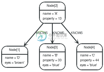
COUNT

COUNTis used to count the number of rows. COUNTcan be used in two forms — COUNT(*)which just counts the number of matching rows, and COUNT(<identifier>), which counts the number of non-nullvalues in <identifier>.

Count nodes

To count the number of nodes, for example the number of nodes connected to one node, you can use count(*).

Query

STARTn=node(2)

MATCH(n)-->(x)

RETURNn, count(*)

This returns the start node and the count of related nodes.

表 . --docbook

n	*count()**
1 row
0 ms
Node[2]{name:"A",property:13}	3

Group Count Relationship Types

To count the groups of relationship types, return the types and count them with count(*).

Query

STARTn=node(2)

MATCH(n)-[r]->()

RETURNtype(r), count(*)

The relationship types and their group count is returned by the query.

表 . --docbook

type(r)	*count()**
1 row
0 ms
"KNOWS"	3

Count entities

Instead of counting the number of results with count(*), it might be more expressive to include the name of the identifier you care about.

Query

STARTn=node(2)

MATCH(n)-->(x)

RETURNcount(x)

The example query returns the number of connected nodes from the start node.

表 . --docbook

count(x)

1 row

0 ms

Count non-null values

You can count the non-nullvalues by using count(<identifier>).

Query

1 2	STARTn=node(2,3,4,1) RETURNcount(n.property?)

The count of related nodes with the propertyproperty set is returned by the query.

表 . --docbook

count(n.property?)

1 row

0 ms

SUM

The SUMaggregation function simply sums all the numeric values it encounters. Nulls are silently dropped. This is an example of how you can use SUM.

Query

1 2	STARTn=node(2,3,4) RETURNsum(n.property)

This returns the sum of all the values in the property property.

表 . --docbook

sum(n.property)

1 row

0 ms

AVG

AVGcalculates the average of a numeric column.

Query

1 2	STARTn=node(2,3,4) RETURNavg(n.property)

The average of all the values in the property propertyis returned by the example query.

表 . --docbook

avg(n.property)

1 row

0 ms

30.0

MAX

MAXfind the largets value in a numeric column.

Query

1 2	STARTn=node(2,3,4) RETURNmax(n.property)

The largest of all the values in the property propertyis returned.

表 . --docbook

max(n.property)

1 row

0 ms

MIN

MINtakes a numeric property as input, and returns the smallest value in that column.

Query

1 2	STARTn=node(2,3,4) RETURNmin(n.property)

This returns the smallest of all the values in the property property.

表 . --docbook

min(n.property)

1 row

0 ms

COLLECT

COLLECTcollects all the values into a list.

Query

1 2	STARTn=node(2,3,4) RETURNcollect(n.property)

Returns a single row, with all the values collected.

表 . --docbook

collect(n.property)

1 row

0 ms

[13,33,44]

DISTINCT

All aggregation functions also take the DISTINCTmodifier, which removes duplicates from the values. So, to count the number of unique eye colors from nodes related to a, this query can be used:

Query

STARTa=node(2)

MATCHa-->b

RETURNcount(distinctb.eyes)

Returns the number of eye colors.

表 . --docbook

count(distinct b.eyes)

1 row

0 ms

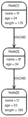
15.8.12. Order by

To sort the output, use the ORDER BYclause. Note that you can not sort on nodes or relationships, just on properties on these.

Graph

Order nodes by property

ORDER BYis used to sort the output.

Query

STARTn=node(3,1,2)

RETURNn

ORDERBYn.name

The nodes are returned, sorted by their name.

表 . --docbook

3 rows

0 ms

Node[1]{name:"A",age:34,length:170}

Node[2]{name:"B",age:34}

Node[3]{name:"C",age:32,length:185}

Order nodes by multiple properties

You can order by multiple properties by stating each identifier in the ORDER BYclause. Cypher will sort the result by the first identifier listed, and for equals values, go to the next property in the ORDER BYclause, and so on.

Query

STARTn=node(3,1,2)

RETURNn

ORDERBYn.age, n.name

This returns the nodes, sorted first by their age, and then by their name.

表 . --docbook

3 rows

0 ms

Node[3]{name:"C",age:32,length:185}

Node[1]{name:"A",age:34,length:170}

Node[2]{name:"B",age:34}

Order nodes in descending order

By adding DESC[ENDING]after the identifier to sort on, the sort will be done in reverse order.

Query

STARTn=node(3,1,2)

RETURNn

ORDERBYn.name DESC

The example returns the nodes, sorted by their name reversely.

表 . --docbook

3 rows

0 ms

Node[3]{name:"C",age:32,length:185}

Node[2]{name:"B",age:34}

Node[1]{name:"A",age:34,length:170}

Ordering null

When sorting the result set, nullwill always come at the end of the result set for ascending sorting, and first when doing descending sort.

Query

STARTn=node(3,1,2)

RETURNn.length?, n

ORDERBYn.length?

The nodes are returned sorted by the length property, with a node without that property last.

表 . --docbook

n.length?	n
3 rows
0 ms
170	Node[1]{name:"A",age:34,length:170}
185	Node[3]{name:"C",age:32,length:185}
<null>	Node[2]{name:"B",age:34}

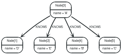
15.8.13. Limit

LIMITenables the return of only subsets of the total result.

Graph

Return first part

To return a subset of the result, starting from the top, use this syntax:

Query

STARTn=node(3, 4, 5, 1, 2)

RETURNn

LIMIT3

The top three items are returned by the example query.

表 . --docbook

3 rows

0 ms

Node[3]{name:"A"}

Node[4]{name:"B"}

Node[5]{name:"C"}

15.8.14. Skip

SKIPenables the return of only subsets of the total result. By using SKIP, the result set will get trimmed from the top. Please note that no guarantees are made on the order of the result unless the query specifies the ORDER BYclause.

Graph

Skip first three

To return a subset of the result, starting from the fourth result, use the following syntax:

Query

STARTn=node(3, 4, 5, 1, 2)

RETURNn

ORDERBYn.name

SKIP3

The first three nodes are skipped, and only the last two are returned in the result.

表 . --docbook

2 rows

0 ms

Node[1]{name:"D"}

Node[2]{name:"E"}

Return middle two

To return a subset of the result, starting from somewhere in the middle, use this syntax:

Query

STARTn=node(3, 4, 5, 1, 2)

RETURNn

ORDERBYn.name

SKIP1

LIMIT2

Two nodes from the middle are returned.

表 . --docbook

2 rows

0 ms

Node[4]{name:"B"}

Node[5]{name:"C"}

15.8.15. With

The ability to chain queries together allows for powerful constructs. In Cypher, the WITHclause is used to pipe the result from one query to the next.

WITHis also used to separate reading from updating of the graph. Every sub-query of a query must be either read-only or write-only.

Graph

Filter on aggregate function results

Aggregated results have to pass through a WITHclause to be able to filter on.

Query

STARTdavid=node(1)

MATCHdavid--otherPerson-->()

WITHotherPerson, count(*) asfoaf

WHEREfoaf > 1

RETURNotherPerson

The person connected to David with the at least more than one outgoing relationship will be returned by the query.

表 . --docbook

otherPerson

1 row

0 ms

Node[3]{name:"Anders"}

Alternative syntax of WITH

If you prefer a more visual way of writing your query, you can use equal-signs as delimiters before and after the column list. Use at least three before the column list, and at least three after.

Query

STARTdavid=node(1)

MATCHdavid--otherPerson-->()

========== otherPerson, count(*) asfoaf ==========

SETotherPerson.connection_count = foaf

For persons connected to David, the connection_countproperty is set to their number of outgoing relationships.

表 . --docbook

Properties set: 2

2 ms

(empty result)

15.8.16. Create

Creating graph elements — nodes and relationships, is done with CREATE.

	提示
	In the CREATEclause, patterns are used a lot. Read 第 15.8 节 “Patterns”for an introduction.

15.8.17. Create single node

Creating a single node is done by issuing the following query.

Query

CREATEn

Nothing is returned from this query, except the count of affected nodes.

表 . --docbook

Nodes created: 1

0 ms

(empty result)

15.8.18. Create single node and set properties

The values for the properties can be any scalar expressions.

Query

1	CREATEn = {name : 'Andres', title : 'Developer'}

Nothing is returned from this query.

表 . --docbook

Nodes created: 1

Properties set: 2

2 ms

(empty result)

15.8.19. Return created node

Creating a single node is done by issuing the following query.

Query

1 2	CREATE(a {name : 'Andres'}) RETURNa

The newly created node is returned. This query uses the alternative syntax for single node creation.

表 . --docbook

1 row

Nodes created: 1

Properties set: 1

3 ms

Node[1]{name:"Andres"}

15.8.20. Create a relationship between two nodes

To create a relationship between two nodes, we first get the two nodes. Once the nodes are loaded, we simply create a relationship between them.

Query

STARTa=node(1), b=node(2)

CREATEa-[r:RELTYPE]->b

RETURNr

The created relationship is returned by the query.

表 . --docbook

1 row

Relationships created: 1

2 ms

:RELTYPE[0] {}

15.8.21. Create a relationship and set properties

Setting properties on relationships is done in a similar manner to how it’s done when creating nodes. Note that the values can be any expression.

Query

STARTa=node(1), b=node(2)

CREATEa-[r:RELTYPE {name : a.name + '<->'+ b.name }]->b

RETURNr

The newly created relationship is returned by the example query.

表 . --docbook

1 row

Relationships created: 1

Properties set: 1

1 ms

:RELTYPE[0] {name:"Andres<->Michael"}

15.8.22. Create a full path

When you use CREATEand a pattern, all parts of the pattern that are not already in scope at this time will be created.

Query

1 2	CREATEp = (andres {name:'Andres'})-[:WORKS_AT]->neo<-[:WORKS_AT]-(michael {name:'Michael'}) RETURNp

This query creates three nodes and two relationships in one go, assigns it to a path identifier, and returns it

表 . --docbook

1 row

Nodes created: 3

Relationships created: 2

Properties set: 2

6 ms

[Node[1]{name:"Andres"},:WORKS_AT[0] {},Node[2]{},:WORKS_AT[1] {},Node[3]{name:"Michael"}]

15.8.23. Create single node from map

You can also create a graph entity from a Map<String,Object>map. All the key/value pairs in the map will be set as properties on the created relationship or node.

Query

1	create({props})

This query can be used in the following fashion:

Map<String, Object> props = newHashMap<String, Object>();

props.put( "name", "Andres");

props.put( "position", "Developer");

Map<String, Object> params = newHashMap<String, Object>();

params.put( "props", props );

engine.execute( "create ({props})", params );

15.8.24. Create multiple nodes from maps

By providing an iterable of maps (Iterable<Map<String,Object>>), Cypher will create a node for each map in the iterable. When you do this, you can’t create anything else in the same create statement.

Query

1	create(n {props}) returnn

This query can be used in the following fashion:

Map<String, Object> n1 = newHashMap<String, Object>();

n1.put( "name", "Andres");

n1.put( "position", "Developer");

Map<String, Object> n2 = newHashMap<String, Object>();

n2.put( "name", "Michael");

n2.put( "position", "Developer");

Map<String, Object> params = newHashMap<String, Object>();

List<Map<String, Object>> maps = Arrays.asList(n1, n2);

params.put( "props", maps);

engine.execute("create (n {props}) return n", params);

15.8.25. Create Unique

CREATE UNIQUEis in the middle of MATCHand CREATE — it will match what it can, and create what is missing. CREATE UNIQUEwill always make the least change possible to the graph — if it can use parts of the existing graph, it will.

Another difference to MATCHis that CREATE UNIQUEassumes the pattern to be unique. If multiple matching subgraphs are found an exception will be thrown.

		提示
In the CREATE UNIQUEclause, patterns are used a lot. Read 第 15.8 节 “Patterns”for an introduction.

15.8.26. Create relationship if it is missing

CREATE UNIQUEis used to describe the pattern that should be found or created.

Query

STARTleft=node(1), right=node(3,4)

CREATEUNIQUEleft-[r:KNOWS]->right

RETURNr

The left node is matched agains the two right nodes. One relationship already exists and can be matched, and the other relationship is created before it is returned.

表 . --docbook

2 rows

Relationships created: 1

4 ms

:KNOWS[4] {}

:KNOWS[3] {}

15.8.27. Create node if missing

If the pattern described needs a node, and it can’t be matched, a new node will be created.

Query

STARTroot=node(2)

CREATEUNIQUEroot-[:LOVES]-someone

RETURNsomeone

The root node doesn’t have any LOVESrelationships, and so a node is created, and also a relationship to that node.

表 . --docbook

someone

1 row

Nodes created: 1

Relationships created: 1

2 ms

Node[5]{}

15.8.28. Create nodes with values

The pattern described can also contain values on the node. These are given using the following syntax: prop : <expression>.

Query

STARTroot=node(2)

CREATEUNIQUEroot-[:X]-(leaf {name:'D'} )

RETURNleaf

No node connected with the root node has the name D, and so a new node is created to match the pattern.

表 . --docbook

leaf

1 row

Nodes created: 1

Relationships created: 1

Properties set: 1

2 ms

Node[5]{name:"D"}

15.8.29. Create relationship with values

Relationships to be created can also be matched on values.

Query

STARTroot=node(2)

CREATEUNIQUEroot-[r:X {since:'forever'}]-()

RETURNr

In this example, we want the relationship to have a value, and since no such relationship can be found, a new node and relationship are created. Note that since we are not interested in the created node, we don’t name it.

表 . --docbook

1 row

Nodes created: 1

Relationships created: 1

Properties set: 1

1 ms

:X[4] {since:"forever"}

15.8.30. Describe complex pattern

The pattern described by CREATE UNIQUEcan be separated by commas, just like in MATCHand CREATE.

Query

STARTroot=node(2)

CREATEUNIQUEroot-[:FOO]->x, root-[:BAR]->x

RETURNx

This example pattern uses two paths, separated by a comma.

表 . --docbook

1 row

Nodes created: 1

Relationships created: 2

10 ms

Node[5]{}

15.8.31. Set

Updating properties on nodes and relationships is done with the SETclause.

15.8.32. Set a property

To set a property on a node or relationship, use SET.

Query

STARTn = node(2)

SETn.surname = 'Taylor'

RETURNn

The newly changed node is returned by the query.

表 . --docbook

1 row

Properties set: 1

1 ms

Node[2]{name:"Andres",age:36,surname:"Taylor"}

15.8.33. Delete

Removing graph elements — nodes, relationships and properties, is done with DELETE.

15.8.34. Delete single node

To remove a node from the graph, you can delete it with the DELETEclause.

Query

1 2	STARTn = node(4) DELETEn

Nothing is returned from this query, except the count of affected nodes.

表 . --docbook

Nodes deleted: 1

15 ms

(empty result)

15.8.35. Remove a node and connected relationships

If you are trying to remove a node with relationships on it, you have to remove these as well.

Query

STARTn = node(3)

MATCHn-[r]-()

DELETEn, r

Nothing is returned from this query, except the count of affected nodes.

表 . --docbook

Nodes deleted: 1

Relationships deleted: 2

1 ms

(empty result)

15.8.36. Remove a property

Neo4j doesn’t allow storing nullin properties. Instead, if no value exists, the property is just not there. So, to remove a property value on a node or a relationship, is also done with DELETE.

Query

STARTandres = node(3)

DELETEandres.age

RETURNandres

The node is returned, and no property ageexists on it.

表 . --docbook

andres

1 row

Properties set: 1

2 ms

Node[3]{name:"Andres"}

15.8.37. Foreach

Collections and paths are key concepts in Cypher. To use them for updating data, you can use the FOREACHconstruct. It allows you to do updating commands on elements in a collection — a path, or a collection created by aggregation.

The identifier context inside of the foreach parenthesis is separate from the one outside it, i.e. if you CREATEa node identifier inside of a FOREACH, you will not be able to use it outside of the foreach statement, unless you match to find it.

Inside of the FOREACHparentheses, you can do any updating commands — CREATE, CREATE UNIQUE, DELETE, and FOREACH.

15.8.38. Mark all nodes along a path

This query will set the property markedto true on all nodes along a path.

Query

STARTbegin = node(2), end = node(1)

MATCHp = begin -[*]-> end foreach(n innodes(p) :

SETn.marked = true)

Nothing is returned from this query.

表 . --docbook

Properties set: 4

2 ms

(empty result)

15.8.39. Functions

Most functions in Cypher will return nullif the input parameter is null.

Here is a list of the functions in Cypher, seperated into three different sections: Predicates, Scalar functions and Aggregated functions

Graph

15.8.40. Predicates

Predicates are boolean functions that return true or false for a given set of input. They are most commonly used to filter out subgraphs in the WHEREpart of a query.

ALL

Tests whether a predicate holds for all element of this collection collection.

Syntax:ALL(identifier in collection WHERE predicate)

Arguments:

- collection:An expression that returns a collection

- identifier:This is the identifier that can be used from the predicate.

- predicate:A predicate that is tested against all items in the collection.

Query

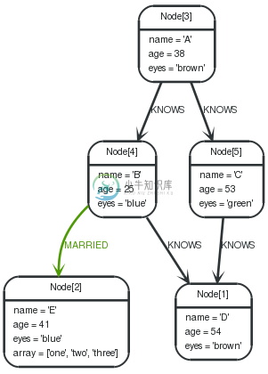
STARTa=node(3), b=node(1)

MATCHp=a-[*1..3]->b

WHEREall(x innodes(p)

WHEREx.age > 30)

RETURNp

All nodes in the returned paths will have an ageproperty of at least 30.

表 . --docbook

1 row

0 ms

[Node[3]{name:"A",age:38,eyes:"brown"},:KNOWS[1] {},Node[5]{name:"C",age:53,eyes:"green"},:KNOWS[3] {},Node[1]{name:"D",age:54,eyes:"brown"}]

ANY

Tests whether a predicate holds for at least one element in the collection.

Syntax:ANY(identifier in collection WHERE predicate)

Arguments:

- collection:An expression that returns a collection

- identifier:This is the identifier that can be used from the predicate.

- predicate:A predicate that is tested against all items in the collection.

Query

STARTa=node(2)

WHEREany(x ina.array

WHEREx = "one")

RETURNa

All nodes in the returned paths has at least one onevalue set in the array property named array.

表 . --docbook

1 row

0 ms

Node[2]{name:"E",age:41,eyes:"blue",array:["one","two","three"]}

NONE

Returns true if the predicate holds for no element in the collection.

Syntax:NONE(identifier in collection WHERE predicate)

Arguments:

- collection:An expression that returns a collection

- identifier:This is the identifier that can be used from the predicate.

- predicate:A predicate that is tested against all items in the collection.

Query

STARTn=node(3)

MATCHp=n-[*1..3]->b

WHERENONE(x innodes(p)

WHEREx.age = 25)

RETURNp

No nodes in the returned paths has a ageproperty set to 25.

表 . --docbook

2 rows

0 ms

[Node[3]{name:"A",age:38,eyes:"brown"},:KNOWS[1] {},Node[5]{name:"C",age:53,eyes:"green"}]

[Node[3]{name:"A",age:38,eyes:"brown"},:KNOWS[1] {},Node[5]{name:"C",age:53,eyes:"green"},:KNOWS[3] {},Node[1]{name:"D",age:54,eyes:"brown"}]

SINGLE

Returns true if the predicate holds for exactly one of the elements in the collection.

Syntax:SINGLE(identifier in collection WHERE predicate)

Arguments:

- collection:An expression that returns a collection

- identifier:This is the identifier that can be used from the predicate.

- predicate:A predicate that is tested against all items in the collection.

Query

STARTn=node(3)

MATCHp=n-->b

WHERESINGLE(var innodes(p)

WHEREvar.eyes = "blue")

RETURNp

Exactly one node in every returned path will have the eyesproperty set to "blue".

表 . --docbook

1 row

0 ms

[Node[3]{name:"A",age:38,eyes:"brown"},:KNOWS[0] {},Node[4]{name:"B",age:25,eyes:"blue"}]

15.8.41. Scalar functions

Scalar functions return a single value.

LENGTH

To return or filter on the length of a collection, use the LENGTH()function.

Syntax:LENGTH( collection )

Arguments:

- collection:An expression that returns a collection

Query

STARTa=node(3)

MATCHp=a-->b-->c

RETURNlength(p)

The length of the path pis returned by the query.

表 . --docbook

length(p)

3 rows

0 ms

TYPE

Returns a string representation of the relationship type.

Syntax:TYPE( relationship )

Arguments:

- relationship:A relationship.

Query

STARTn=node(3)

MATCH(n)-[r]->()

RETURNtype(r)

The relationship type of ris returned by the query.

表 . --docbook

type(r)

2 rows

0 ms

"KNOWS"

Returns the id of the relationship or node.

Syntax:ID( property-container )

Arguments:

- property-container:A node or a relationship.

Query

1 2	STARTa=node(3, 4, 5) RETURNID(a)

This returns the node id for three nodes.

表 . --docbook

ID(a)

3 rows

0 ms

COALESCE

Returns the first non-nullvalue in the list of expressions passed to it.

Syntax:COALESCE( expression [, expression]* )

Arguments:

- expression:The expression that might return null.

Query

1 2	STARTa=node(3) RETURNcoalesce(a.hairColour?, a.eyes?)

表 . --docbook

coalesce(a.hairColour?, a.eyes?)

1 row

0 ms

"brown"

HEAD

HEADreturns the first element in a collection.

Syntax:HEAD( expression )

Arguments:

- expression:This expression should return a collection of some kind.

Query

1 2	STARTa=node(2) RETURNa.array, head(a.array)

The first node in the path is returned.

表 . --docbook

a.array	head(a.array)
1 row
0 ms
["one","two","three"]	"one"

LAST

LASTreturns the last element in a collection.

Syntax:LAST( expression )

Arguments:

- expression:This expression should return a collection of some kind.

Query

1 2	STARTa=node(2) RETURNa.array, last(a.array)

The last node in the path is returned.

表 . --docbook

a.array	last(a.array)
1 row
0 ms
["one","two","three"]	"three"

15.8.42. Collection functions

Collection functions return collections of things — nodes in a path, and so on.

NODES

Returns all nodes in a path.

Syntax:NODES( path )

Arguments:

- path:A path.

Query

STARTa=node(3), c=node(2)

MATCHp=a-->b-->c

RETURNNODES(p)

All the nodes in the path pare returned by the example query.

表 . --docbook

NODES(p)

1 row

0 ms

[Node[3]{name:"A",age:38,eyes:"brown"},Node[4]{name:"B",age:25,eyes:"blue"},Node[2]{name:"E",age:41,eyes:"blue",array:["one","two","three"]}]

RELATIONSHIPS

Returns all relationships in a path.

Syntax:RELATIONSHIPS( path )

Arguments:

- path:A path.

Query

STARTa=node(3), c=node(2)

MATCHp=a-->b-->c

RETURNRELATIONSHIPS(p)

All the relationships in the path pare returned.

表 . --docbook

RELATIONSHIPS(p)

1 row

0 ms

[:KNOWS[0] {},:MARRIED[4] {}]

EXTRACT

To return a single property, or the value of a function from a collection of nodes or relationships, you can use EXTRACT. It will go through a collection, run an expression on every element, and return the results in an collection with these values. It works like the mapmethod in functional languages such as Lisp and Scala.

Syntax:EXTRACT( identifier in collection : expression )

Arguments:

- collection:An expression that returns a collection

- identifier:The closure will have an identifier introduced in it’s context. Here you decide which identifier to use.

- expression:This expression will run once per value in the collection, and produces the result collection.

Query

STARTa=node(3), b=node(4), c=node(1)

MATCHp=a-->b-->c

RETURNextract(n innodes(p) : n.age)

The age property of all nodes in the path are returned.

表 . --docbook

extract(n in nodes(p) : n.age)

1 row

0 ms

[38,25,54]

FILTER

FILTERreturns all the elements in a collection that comply to a predicate.

Syntax:FILTER(identifier in collection : predicate)

Arguments:

- collection:An expression that returns a collection

- identifier:This is the identifier that can be used from the predicate.

- predicate:A predicate that is tested against all items in the collection.

Query

1 2	STARTa=node(2) RETURNa.array, filter(x ina.array : length(x) = 3)

This returns the property named arrayand a list of values in it, which have the length 3.

表 . --docbook

a.array	filter(x in a.array : length(x) = 3)
1 row
0 ms
["one","two","three"]	["one","two"]

TAIL

TAILreturns all but the first element in a collection.

Syntax:TAIL( expression )

Arguments:

- expression:This expression should return a collection of some kind.

Query

1 2	STARTa=node(2) RETURNa.array, tail(a.array)

This returns the property named arrayand all elements of that property except the first one.

表 . --docbook

a.array	tail(a.array)
1 row
0 ms
["one","two","three"]	["two","three"]

RANGE

Returns numerical values in a range with a non-zero step value step. Range is inclusive in both ends.

Syntax:RANGE( start, end [, step] )

Arguments:

- start:A numerical expression.

- end:A numerical expression.

- step:A numerical expression.

Query

1 2	STARTn=node(1) RETURNrange(0,10), range(2,18,3)

Two lists of numbers are returned.

表 . --docbook

range(0,10)	range(2,18,3)
1 row
0 ms
[0,1,2,3,4,5,6,7,8,9,10]	[2,5,8,11,14,17]

15.8.43. Mathematical functions

These functions all operate on numerical expressions only, and will return an error if used on any other values.

ABS

ABSreturns the absolute value of a number.

Syntax:ABS( expression )

Arguments:

- expression:A numeric expression.

Query

1 2	STARTa=node(3), c=node(2) RETURNa.age, c.age, abs(a.age - c.age)

The absolute value of the age difference is returned.

表 . --docbook

a.age	c.age	abs(a.age - c.age)
1 row
0 ms
38	41	3.0

ROUND

ROUNDreturns the numerical expression, rounded to the nearest integer.

Syntax:ROUND( expression )

Arguments:

- expression:A numerical expression.

Query

1 2	STARTa=node(1) RETURNround(3.141592)

表 . --docbook

round(3.141592)

1 row

0 ms

SQRT

SQRTreturns the square root of a number.

Syntax:SQRT( expression )

Arguments:

- expression:A numerical expression

Query

1 2	STARTa=node(1) RETURNsqrt(256)

表 . --docbook

sqrt(256)

1 row

0 ms

SIGN

SIGNreturns the signum of a number — zero if the expression is zero, -1for any negative number, and 1for any positive number.

Syntax:SIGN( expression )

Arguments:

- expression:A numerical expression

Query

1 2	STARTn=node(1) RETURNsign(-17), sign(0.1)

表 . --docbook

sign(-17)	sign(0.1)
1 row
0 ms
-1.0	1.0

15.8.44. 兼容性

Cypher is still changing rather rapidly. Parts of the changes are internal — we add new pattern matchers, aggregators and other optimizations, which hopefully makes your queries run faster.

Other changes are directly visible to our users — the syntax is still changing. New concepts are being added and old ones changed to fit into new possibilities. To guard you from having to keep up with our syntax changes, Cypher allows you to use an older parser, but still gain the speed from new optimizations.

There are two ways you can select which parser to use. You can configure your database with the configuration parameter cypher_parser_version, and enter which parser you’d like to use (1.6, 1.7 and 1.8 are supported now). Any Cypher query that doesn’t explicitly say anything else, will get the parser you have configured.

The other way is on a query by query basis. By simply pre-pending your query with "CYPHER 1.6", that particular query will be parsed with the 1.6 version of the parser. Example:

CYPHER1.6 STARTn=node(0)

WHEREn.foo = "bar"

RETURNn

15.8.45. 从SQL到Cypher查询

This guide is for people who understand SQL. You can use that prior knowledge to quickly get going with Cypher and start exploring Neo4j.

Start

SQL starts with the result you want — we SELECTwhat we want and then declare how to source it. In Cypher, the STARTclause is quite a different concept which specifies starting points in the graph from which the query will execute.

From a SQL point of view, the identifiers in STARTare like table names that point to a set of nodes or relationships. The set can be listed literally, come via parameters, or as I show in the following example, be defined by an index look-up.

So in fact rather than being SELECT-like, the STARTclause is somewhere between the FROMand the WHEREclause in SQL.

SQL Query.

SELECT*

FROM"Person"

WHEREname= 'Anakin'

表 . --docbook

NAME	ID	AGE	HAIR
1 rows
Anakin	1	20	blonde

Cypher Query.

1 2	STARTperson=node:Person(name = 'Anakin') RETURNperson

表 . --docbook

person

1 row

1 ms

Node[1]{name:"Anakin",id:1,age:20,hair:"blonde"}

Cypher allows multiple starting points. This should not be strange from a SQL perspective — every table in the FROMclause is another starting point.

Match

Unlike SQL which operates on sets, Cypher predominantly works on sub-graphs. The relational equivalent is the current set of tuples being evaluated during a SELECTquery.

The shape of the sub-graph is specified in the MATCHclause. The MATCHclause is analogous to the JOINin SQL. A normal a→b relationship is an inner join between nodes a and b — both sides have to have at least one match, or nothing is returned.

We’ll start with a simple example, where we find all email addresses that are connected to the person “Anakin”. This is an ordinary one-to-many relationship.

SQL Query.

SELECT"Email".*

FROM"Person"

JOIN"Email"ON"Person".id = "Email".person_id

WHERE"Person".name= 'Anakin'

表 . --docbook

ADDRESS	COMMENT	PERSON_ID
2 rows
anakin@example.com	home	1
anakin@example.org	work	1

Cypher Query.

STARTperson=node:Person(name = 'Anakin')

MATCHperson-[:email]->email

RETURNemail

表 . --docbook

email

2 rows

11 ms

Node[7]{address:"anakin@example.com",comment:"home"}

Node[8]{address:"anakin@example.org",comment:"work"}

在这里，没有联接表，但如果一个必要下一个示例将显示如何做到这一点，写作模式的关系像这样：-[r: belongs_to]-> 将介绍（相当于）联接表可用作变量 r。在现实中这是命名的关系，在加密，所以我们说"belongs_to 通过加入人到组"。为了说明这一点，请考虑此图像，比较 SQL 模型和 Neo4j/暗号表达。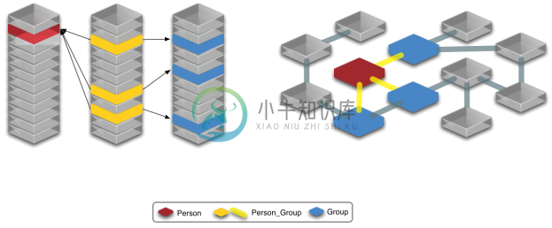

And here are example queries:

SQL Query.

SELECT"Group".*, "Person_Group".*

FROM"Person"

JOIN"Person_Group"ON"Person".id = "Person_Group".person_id

JOIN"Group"ON"Person_Group".Group_id="Group".id

WHERE"Person".name= 'Bridget'

表 . --docbook

NAME	ID	BELONGS_TO_GROUP_ID	PERSON_ID	GROUP_ID
1 rows
Admin	4	3	2	4

Cypher Query.

STARTperson=node:Person(name = 'Bridget')

MATCHperson-[r:belongs_to]->group

RETURNgroup, r

表 . --docbook

group	r
1 row
0 ms
Node[6]{name:"Admin",id:4}	:belongs_to[0] {}

An outer joinis just as easy. Add a question mark -[?:KNOWS]->and it’s an optional relationship between nodes — the outer join of Cypher.

Whether it’s a left outer join, or a right outer join is defined by which side of the pattern has a starting point. This example is a left outer join, because the bound node is on the left side:

SQL Query.

SELECT"Person".name, "Email".address

FROM"Person"LEFT

JOIN"Email"ON"Person".id = "Email".person_id

表 . --docbook

NAME	ADDRESS
3 rows
Anakin	anakin@example.com
Anakin	anakin@example.org
Bridget	<null>

Cypher Query.

STARTperson=node:Person('name: *')

MATCHperson-[?:email]->email

RETURNperson.name, email.address?

表 . --docbook

person.name	email.address?
3 rows
3 ms
"Anakin"	"anakin@example.com"
"Anakin"	"anakin@example.org"
"Bridget"	<null>

Relationships in Neo4j are first class citizens — it’s like the SQL tables are pre-joined with each other. So, naturally, Cypher is designed to be able to handle highly connected data easily.

One such domain is tree structures — anyone that has tried storing tree structures in SQL knows that you have to work hard to get around the limitations of the relational model. There are even books on the subject.

To find all the groups and sub-groups that Bridget belongs to, this query is enough in Cypher:

Cypher Query.

STARTperson=node:Person('name: Bridget')

MATCHperson-[:belongs_to*]->group

RETURNperson.name, group.name

表 . --docbook

person.name	group.name
3 rows
4 ms
"Bridget"	"Admin"
"Bridget"	"Technichian"
"Bridget"	"User"

The * after the relationship type means that there can be multiple hops across belongs_torelationships between group and user. Some SQL dialects have recursive abilities, that allow the expression of queries like this, but you may have a hard time wrapping your head around those. Expressing something like this in SQL is hugely impractical if not practically impossible.

Where

This is the easiest thing to understand — it’s the same animal in both languages. It filters out result sets/subgraphs. Not all predicates have an equivalent in the other language, but the concept is the same.

SQL Query.

SELECT*

FROM"Person"

WHERE"Person".age > 35 AND"Person".hair = 'blonde'

表 . --docbook

NAME	ID	AGE	HAIR
1 rows
Bridget	2	40	blonde

Cypher Query.

STARTperson=node:Person('name: *')

WHEREperson.age > 35 ANDperson.hair = 'blonde'

RETURNperson

表 . --docbook

person

1 row

3 ms

Node[2]{name:"Bridget",id:2,age:40,hair:"blonde"}

Return

This is SQL’s SELECT. We just put it in the end because it felt better to have it there — you do a lot of matching and filtering, and finally, you return something.

Aggregate queries work just like they do in SQL, apart from the fact that there is no explicit GROUP BYclause. Everything in the return clause that is not an aggregate function will be used as the grouping columns.

SQL Query.

SELECT"Person".name, count(*)

FROM"Person"

GROUPBY"Person".name

ORDERBY"Person".name

表 . --docbook

NAME	C2
2 rows
Anakin	1
Bridget	1

Cypher Query.

STARTperson=node:Person('name: *')

RETURNperson.name, count(*)

ORDERBYperson.name

表 . --docbook

person.name	*count()**
2 rows
1 ms
"Anakin"	1
"Bridget"	1

Order by is the same in both languages — ORDER BYexpression ASC/DESC. Nothing weird here.