TensorFlow实现Batch Normalization

一、BN（Batch Normalization）算法

1. 对数据进行归一化处理的重要性

神经网络学习过程的本质就是学习数据分布，在训练数据与测试数据分布不同情况下，模型的泛化能力就大大降低；另一方面，若训练过程中每批batch的数据分布也各不相同，那么网络每批迭代学习过程也会出现较大波动，使之更难趋于收敛，降低训练收敛速度。对于深层网络，网络前几层的微小变化都会被网络累积放大，则训练数据的分布变化问题会被放大，更加影响训练速度。

2. BN算法的强大之处

1）为了加速梯度下降算法的训练，我们可以采取指数衰减学习率等方法在初期快速学习，后期缓慢进入全局最优区域。使用BN算法后，就可以直接选择比较大的学习率，且设置很大的学习率衰减速度，大大提高训练速度。即使选择了较小的学习率，也会比以前不使用BN情况下的收敛速度快。总结就是BN算法具有快速收敛的特性。

2）BN具有提高网络泛化能力的特性。采用BN算法后，就可以移除针对过拟合问题而设置的dropout和L2正则化项，或者采用更小的L2正则化参数。

3）BN本身是一个归一化网络层，则局部响应归一化层（Local Response Normalization，LRN层）则可不需要了（Alexnet网络中使用到）。

3. BN算法概述

BN算法提出了变换重构，引入了可学习参数γ、β，这就是算法的关键之处：

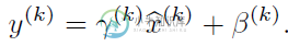
引入这两个参数后，我们的网络便可以学习恢复出原是网络所要学习的特征分布，BN层的钱箱传到过程如下：

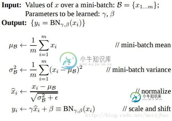
其中m为batchsize。BatchNormalization中所有的操作都是平滑可导，这使得back propagation可以有效运行并学到相应的参数γ，β。需要注意的一点是Batch Normalization在training和testing时行为有所差别。Training时μβ和σβ由当前batch计算得出；在Testing时μβ和σβ应使用Training时保存的均值或类似的经过处理的值，而不是由当前batch计算。

二、TensorFlow相关函数

1.tf.nn.moments(x, axes, shift=None, name=None, keep_dims=False)

x是输入张量，axes是在哪个维度上求解， 即想要 normalize的维度, [0] 代表 batch 维度，如果是图像数据，可以传入 [0, 1, 2]，相当于求[batch, height, width] 的均值/方差，注意不要加入channel 维度。该函数返回两个张量，均值mean和方差variance。

2.tf.identity(input, name=None)

返回与输入张量input形状和内容一致的张量。

3.tf.nn.batch_normalization(x, mean, variance, offset, scale, variance_epsilon,name=None)

计算公式为scale(x - mean)/ variance + offset。

这些参数中，tf.nn.moments可得到均值mean和方差variance，offset和scale是可训练的，offset一般初始化为0，scale初始化为1，offset和scale的shape与mean相同，variance_epsilon参数设为一个很小的值如0.001。

三、TensorFlow代码实现

1. 完整代码

import tensorflow as tf 
import numpy as np 
import matplotlib.pyplot as plt 
 
ACTIVITION = tf.nn.relu 
N_LAYERS = 7 # 总共7层隐藏层 
N_HIDDEN_UNITS = 30 # 每层包含30个神经元 
 
def fix_seed(seed=1): # 设置随机数种子 
  np.random.seed(seed) 
  tf.set_random_seed(seed) 
 
def plot_his(inputs, inputs_norm): # 绘制直方图函数 
  for j, all_inputs in enumerate([inputs, inputs_norm]): 
    for i, input in enumerate(all_inputs): 
      plt.subplot(2, len(all_inputs), j*len(all_inputs)+(i+1)) 
      plt.cla() 
      if i == 0: 
        the_range = (-7, 10) 
      else: 
        the_range = (-1, 1) 
      plt.hist(input.ravel(), bins=15, range=the_range, color='#FF5733') 
      plt.yticks(()) 
      if j == 1: 
        plt.xticks(the_range) 
      else: 
        plt.xticks(()) 
      ax = plt.gca() 
      ax.spines['right'].set_color('none') 
      ax.spines['top'].set_color('none') 
    plt.title("%s normalizing" % ("Without" if j == 0 else "With")) 
  plt.draw() 
  plt.pause(0.01) 
 
def built_net(xs, ys, norm): # 搭建网络函数 
  # 添加层 
  def add_layer(inputs, in_size, out_size, activation_function=None, norm=False): 
    Weights = tf.Variable(tf.random_normal([in_size, out_size], 
                        mean=0.0, stddev=1.0)) 
    biases = tf.Variable(tf.zeros([1, out_size]) + 0.1) 
    Wx_plus_b = tf.matmul(inputs, Weights) + biases 
 
    if norm: # 判断是否是Batch Normalization层 
      # 计算均值和方差，axes参数0表示batch维度 
      fc_mean, fc_var = tf.nn.moments(Wx_plus_b, axes=[0]) 
      scale = tf.Variable(tf.ones([out_size])) 
      shift = tf.Variable(tf.zeros([out_size])) 
      epsilon = 0.001 
 
      # 定义滑动平均模型对象 
      ema = tf.train.ExponentialMovingAverage(decay=0.5) 
 
      def mean_var_with_update(): 
        ema_apply_op = ema.apply([fc_mean, fc_var]) 
        with tf.control_dependencies([ema_apply_op]): 
          return tf.identity(fc_mean), tf.identity(fc_var) 
 
      mean, var = mean_var_with_update() 
 
      Wx_plus_b = tf.nn.batch_normalization(Wx_plus_b, mean, var, 
                         shift, scale, epsilon) 
 
    if activation_function is None: 
      outputs = Wx_plus_b 
    else: 
      outputs = activation_function(Wx_plus_b) 
    return outputs 
 
  fix_seed(1) 
 
  if norm: # 为第一层进行BN 
    fc_mean, fc_var = tf.nn.moments(xs, axes=[0]) 
    scale = tf.Variable(tf.ones([1])) 
    shift = tf.Variable(tf.zeros([1])) 
    epsilon = 0.001 
 
    ema = tf.train.ExponentialMovingAverage(decay=0.5) 
 
    def mean_var_with_update(): 
      ema_apply_op = ema.apply([fc_mean, fc_var]) 
      with tf.control_dependencies([ema_apply_op]): 
        return tf.identity(fc_mean), tf.identity(fc_var) 
 
    mean, var = mean_var_with_update() 
    xs = tf.nn.batch_normalization(xs, mean, var, shift, scale, epsilon) 
 
  layers_inputs = [xs] # 记录每一层的输入 
 
  for l_n in range(N_LAYERS): # 依次添加7层 
    layer_input = layers_inputs[l_n] 
    in_size = layers_inputs[l_n].get_shape()[1].value 
 
    output = add_layer(layer_input, in_size, N_HIDDEN_UNITS, ACTIVITION, norm) 
    layers_inputs.append(output) 
 
  prediction = add_layer(layers_inputs[-1], 30, 1, activation_function=None) 
  cost = tf.reduce_mean(tf.reduce_sum(tf.square(ys - prediction), 
                    reduction_indices=[1])) 
 
  train_op = tf.train.GradientDescentOptimizer(0.001).minimize(cost) 
  return [train_op, cost, layers_inputs] 
 
fix_seed(1) 
x_data = np.linspace(-7, 10, 2500)[:, np.newaxis] 
np.random.shuffle(x_data) 
noise =np.random.normal(0, 8, x_data.shape) 
y_data = np.square(x_data) - 5 + noise 
 
plt.scatter(x_data, y_data) 
plt.show() 
 
xs = tf.placeholder(tf.float32, [None, 1]) 
ys = tf.placeholder(tf.float32, [None, 1]) 
 
train_op, cost, layers_inputs = built_net(xs, ys, norm=False) 
train_op_norm, cost_norm, layers_inputs_norm = built_net(xs, ys, norm=True) 
 
with tf.Session() as sess: 
  sess.run(tf.global_variables_initializer()) 
 
  cost_his = [] 
  cost_his_norm = [] 
  record_step = 5 
 
  plt.ion() 
  plt.figure(figsize=(7, 3)) 
  for i in range(250): 
    if i % 50 == 0: 
      all_inputs, all_inputs_norm = sess.run([layers_inputs, layers_inputs_norm], 
                          feed_dict={xs: x_data, ys: y_data}) 
      plot_his(all_inputs, all_inputs_norm) 
 
    sess.run([train_op, train_op_norm], 
         feed_dict={xs: x_data[i*10:i*10+10], ys: y_data[i*10:i*10+10]}) 
 
    if i % record_step == 0: 
      cost_his.append(sess.run(cost, feed_dict={xs: x_data, ys: y_data})) 
      cost_his_norm.append(sess.run(cost_norm, 
                     feed_dict={xs: x_data, ys: y_data})) 
 
  plt.ioff() 
  plt.figure() 
  plt.plot(np.arange(len(cost_his))*record_step, 
       np.array(cost_his), label='Without BN')   # no norm 
  plt.plot(np.arange(len(cost_his))*record_step, 
       np.array(cost_his_norm), label='With BN')  # norm 
  plt.legend() 
  plt.show() 

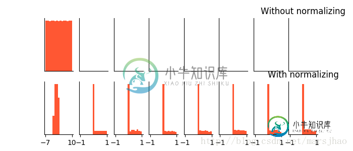
2. 实验结果

输入数据分布：

批标准化BN效果对比：

以上就是本文的全部内容，希望对大家的学习有所帮助，也希望大家多多支持小牛知识库。