具有张量流概率的贝叶斯线性回归

Question

我无法让贝叶斯线性回归与Tensorflow概率一起使用。这是我的代码：

!pip install tensorflow==2.0.0-rc1
!pip install tensorflow-probability==0.8.0rc0

import numpy as np
import tensorflow as tf
import tensorflow_probability as tfp
tfd = tfp.distributions
N = 20
std = 1
m = np.random.normal(0, scale=5, size=1).astype(np.float32)
b = np.random.normal(0, scale=5, size=1).astype(np.float32)
x = np.linspace(0, 100, N).astype(np.float32)
y = m*x+b+ np.random.normal(loc=0, scale=std, size=N).astype(np.float32)

num_results = 10000
num_burnin_steps = 5000

def joint_log_prob(x, y, m, b, std):
  rv_m = tfd.Normal(loc=0, scale=5)
  rv_b = tfd.Normal(loc=0, scale=5)
  rv_std = tfd.HalfCauchy(loc=0., scale=2.)

  y_mu = m*x+b
  rv_y = tfd.Normal(loc=y_mu, scale=std)

  return (rv_m.log_prob(m) + rv_b.log_prob(b) + rv_std.log_prob(std)
          + tf.reduce_sum(rv_y.log_prob(y)))

# Define a closure over our joint_log_prob.
def target_log_prob_fn(m, b, std):
    return joint_log_prob(x, y, m, b, std)

@tf.function(autograph=False)
def do_sampling():
  kernel=tfp.mcmc.HamiltonianMonteCarlo(
          target_log_prob_fn=target_log_prob_fn,
          step_size=0.05,
          num_leapfrog_steps=3)
  kernel = tfp.mcmc.SimpleStepSizeAdaptation(
        inner_kernel=kernel, num_adaptation_steps=int(num_burnin_steps * 0.8))
  return tfp.mcmc.sample_chain(
      num_results=num_results,
      num_burnin_steps=num_burnin_steps,
      current_state=[
          0.01 * tf.ones([], name='init_m', dtype=tf.float32),
          0.01 * tf.ones([], name='init_b', dtype=tf.float32),
          1 * tf.ones([], name='init_std', dtype=tf.float32)
      ],
      kernel=kernel,
      trace_fn=lambda _, pkr: [pkr.inner_results.accepted_results.step_size,
                               pkr.inner_results.log_accept_ratio])

samples, [step_size, log_accept_ratio] = do_sampling()
m_posterior, b_posterior, std_posterior = samples

p_accept = tf.reduce_mean(tf.exp(tf.minimum(log_accept_ratio, 0.)))
print('Acceptance rate: {}'.format(p_accept))

n_v = len(samples)
true_values = [m, b, std]

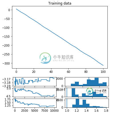
plt.figure()
plt.title('Training data')
plt.plot(x, y)

plt.figure()
plt.title('Visualizing trace and posterior distributions')
for i, (sample, true_value) in enumerate(zip(samples, true_values)):
  plt.subplot(2*n_v, 2, 2*i+1)
  plt.plot(sample)
  plt.subplot(2*n_v, 2, 2*i+2)
  plt.hist(sample)
  plt.axvline(x=true_value)
>>> Acceptance rate: 0.006775229703634977

有什么想法吗？

Answer 1

首先，这个问题提出得很好——我很容易复制/粘贴您的代码并重新生成：）

第一个问题（与 HMC 一样）是step_size/num_leapfrog_steps设置。我能够通过使步长更小（~.007）和跳跃步长更少（~3）来获得不错的接受率（~.7）。通常，您希望将蛙跳步保持在您可以管理的范围内尽可能小，因为每个步骤都会导致昂贵的梯度计算。

下一个问题是，看起来链与这些参数的混合仍然不太好。我怀疑这可能是居中与非中心（参见 https://discourse.mc-stan.org/t/centered-vs-noncentered/1502）参数化的问题;你可能有更好的运气改变模型的参数化，尽管我不是很熟悉这个的细节...

为了自动找到更好的步长参数，您可以尝试两个步长自适应内核中的一个——SimpleStepSizeAdaptation或DualAveragingStepSize Adaptatation——可以围绕HMC内核实例进行包装。此外，您可以尝试使用NoUTurnSampler作为vanilla HMC的替代方案，以避免必须调整蛙跳步骤参数。对于一个简单的贝叶斯线性回归示例来说，所有这些都是非常重要的，但我想这个示例强调了正确地处理MCMC是多么困难：）

希望这有帮助！请随时发送消息给我们[e-mail]更多的讨论——也许其他一些对参数化问题有更多了解的人会加入进来。再次感谢你提出这个好问题。

Answer 2

令人惊讶的是，这样一个简单的问题竟然如此困难！原始 HMC 在设置推理时对相对较小的细节可能非常敏感。像斯坦这样的系统试图通过为你做大量的调优来处理这个问题，但TFP的自动调谐现在要基本得多。

我在这里发现了一些似乎可以很好地进行推理的变化。简而言之，它们是：

• 在不受约束的空间中重新参数化。
• 使用非均匀步长（相当于：添加对角线预条件器）
• 增加HMC越级步数。
• 使用DualAveragingStepSizeAdapation而不是SimpleStepSizeAdapation。

第一个技巧是使用TransformedTrantionKernel进行重新参数化，使度参数存在于不受约束的空间中。例如，我们可以使用Expbijector来定义log-scale参数：

tfb = tfp.bijectors
kernel = tfp.mcmc.TransformedTransitionKernel(
      inner_kernel=kernel,
      bijector=[tfb.Identity(), tfb.Identity(), tfb.Exp()]
  )

这确保了推理只考虑标度的正值，所以它不必拒绝使标度小于零的每个移动。当我这样做的时候，接受率上升了，尽管混合仍然不是很好。

第二个变化是对三个变量使用不一致的步长(这相当于对角预处理)。看起来这个模型中的后验概率是病态的:二十个数据点确定斜率比它们确定截距或标度要精确得多。TFP中的“步长自适应”简单地找到一个步长，使得指定百分比的样本被接受，这通常由最严格约束的后验分量控制:如果其他分量具有宽得多的后验，小的步长将防止它们混合。估计合理步长的一种方法是使用变分推断的标准偏差和分解的正态替代后验概率:

surrogate_posterior = tfp.experimental.vi.build_factored_surrogate_posterior(
    event_shape=[[], [], []],
    constraining_bijectors=[None, None, tfb.Exp()])
losses = tfp.vi.fit_surrogate_posterior(
    target_log_prob_fn, surrogate_posterior,
    optimizer=tf.optimizers.Adam(
        learning_rate=0.1,
        # Decay second-moment estimates to aid optimizing scale parameters.
        beta_2=0.9),
    num_steps=1000)
approximate_posterior_stddevs = [np.std(x) for x in surrogate_posterior.sample(50)]

另一个普遍的技巧是增加蛙跳的步数。考虑HMC的一种方式是，在蛙跳积分器中，它类似于一个具有动量的优化器，但它在每次停止接受/拒绝时都会失去动量(通过重新采样)。因此，在我们每步都这样做的极端情况下(< code > num _ leapfrog _ steps = 1 ，即Langevin dynamics)，无论如何都没有动量，增加leap frog步骤的数量往往会提高导航复杂几何图形的能力，类似于动量如何提高优化器。我没有严格地调优任何东西，但是将< code > num _ leap frog _ steps = 16 设置为3似乎有很大帮助。

这是我修改后的代码版本，包含了这些技巧。它似乎在大多数执行中混合得很好（尽管我确信它并不完美）：

!pip install tensorflow==2.0.0-rc1
!pip install tensorflow-probability==0.8.0rc0

import numpy as np
import tensorflow as tf
import tensorflow_probability as tfp

tfd = tfp.distributions
tfb = tfp.bijectors

N = 20
std = 1
m = np.random.normal(0, scale=5, size=1).astype(np.float32)
b = np.random.normal(0, scale=5, size=1).astype(np.float32)
x = np.linspace(0, 100, N).astype(np.float32)
y = m*x+b+ np.random.normal(loc=0, scale=std, size=N).astype(np.float32)

num_results = 1000
num_burnin_steps = 500

def joint_log_prob(x, y, m, b, std):
  rv_m = tfd.Normal(loc=0, scale=5)
  rv_b = tfd.Normal(loc=0, scale=5)
  rv_std = tfd.HalfCauchy(0., scale=1.)

  y_mu = m*x+b
  rv_y = tfd.Normal(loc=y_mu, scale=rv_std[..., None])

  return (rv_m.log_prob(m) + rv_b.log_prob(b)
          + rv_std.log_prob(std)
          + tf.reduce_sum(rv_y.log_prob(y)))

# Define a closure over our joint_log_prob.
def target_log_prob_fn(m, b, std):
    return joint_log_prob(x, y, m, b, std)

# Run variational inference to initialize per-variable step sizes.
surrogate_posterior = tfp.experimental.vi.build_factored_surrogate_posterior(
    event_shape=[[], [], []],
    constraining_bijectors=[None, None, tfb.Exp()])
losses = tfp.vi.fit_surrogate_posterior(
    target_log_prob_fn,
    surrogate_posterior,
    optimizer=tf.optimizers.Adam(
        learning_rate=0.1,
        # Decay second-moment estimates to aid optimizing scale parameters.
        beta_2=0.9),
    num_steps=1000)
approximate_posterior_stddevs = [np.std(z) for z in surrogate_posterior.sample(50)]

@tf.function(autograph=False)
def do_sampling():
  kernel=tfp.mcmc.HamiltonianMonteCarlo(
          target_log_prob_fn=target_log_prob_fn,
          step_size=approximate_posterior_stddevs,
          num_leapfrog_steps=16)
  kernel = tfp.mcmc.TransformedTransitionKernel(
      inner_kernel=kernel,
      bijector=[tfb.Identity(),
                tfb.Identity(),
                tfb.Exp()]
  )
  kernel = tfp.mcmc.DualAveragingStepSizeAdaptation(
        inner_kernel=kernel,
        num_adaptation_steps=int(num_burnin_steps * 0.8))
  return tfp.mcmc.sample_chain(
      num_results=num_results,
      num_burnin_steps=num_burnin_steps,
      current_state=[
          0.01 * tf.ones([], name='init_m', dtype=tf.float32),
          0.01 * tf.ones([], name='init_b', dtype=tf.float32),
          1. * tf.ones([], name='init_std', dtype=tf.float32)
      ],
      kernel=kernel,
      trace_fn=lambda _, pkr: [pkr.inner_results.inner_results.accepted_results.step_size,
                               pkr.inner_results.inner_results.log_accept_ratio])

samples, [step_size, log_accept_ratio] = do_sampling()
m_posterior, b_posterior, std_posterior = samples

p_accept = tf.reduce_mean(tf.exp(tf.minimum(log_accept_ratio, 0.)))
print('Acceptance rate: {}'.format(p_accept))

n_v = len(samples)
true_values = [m, b, std]

plt.figure(figsize=(12, 12))
plt.title('Visualizing trace and posterior distributions')
for i, (sample, true_value) in enumerate(zip(samples, true_values)):
  plt.subplot(2*n_v, 2, 2*i+1)
  plt.plot(sample)
  plt.subplot(2*n_v, 2, 2*i+2)
  plt.hist(sample.numpy())
  plt.axvline(x=true_value)