Science Plots
Matplotlib styles for scientific figures
This repo has Matplotlib styles to format your figures for scientific papers, presentations and theses.
Getting Started
The easiest way to install SciencePlots is by using pip:
# to install the lastest release (from PyPI)
pip install SciencePlots==1.0.9

# to install the latest commit (from GitHub)
pip install git+https://github.com/garrettj403/SciencePlots

# to clone and then install from a local copy
git clone https://github.com/garrettj403/SciencePlots.git
cd SciencePlots
pip install -e .
The pip installation will automatically move all of the Matplotlib style files *.mplstyle into the appropriate directory on your computer.
Notes:
- SciencePlots requires Latex (see Latex installation instructions).
- If you would like to use CJK fonts, you will need to install these font separately (see CJK font installation instructions).
Please see the FAQ section for more information and troubleshooting.
Using the Styles
"science" is the main style from this repo. Whenever you want to use it, simply add the following to the top of your python script:
import matplotlib.pyplot as plt

plt.style.use('science')
You can also combine multiple styles together by:
plt.style.use(['science','ieee'])
In this case, the ieee style will override some of the parameters from the science style in order to configure the plot for IEEE papers (column width, fontsizes, etc.).
To use any of the styles temporarily, you can use:
with plt.style.context(['science', 'ieee']):
    plt.figure()
    plt.plot(x, y)
    plt.show()
Examples
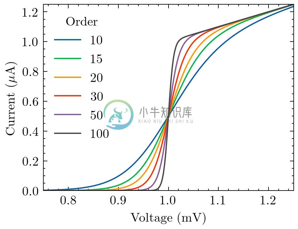
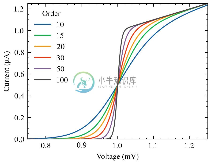
The science style:
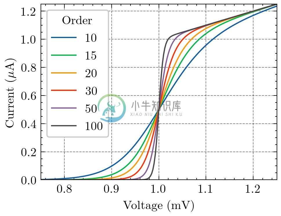
The science + grid styles:
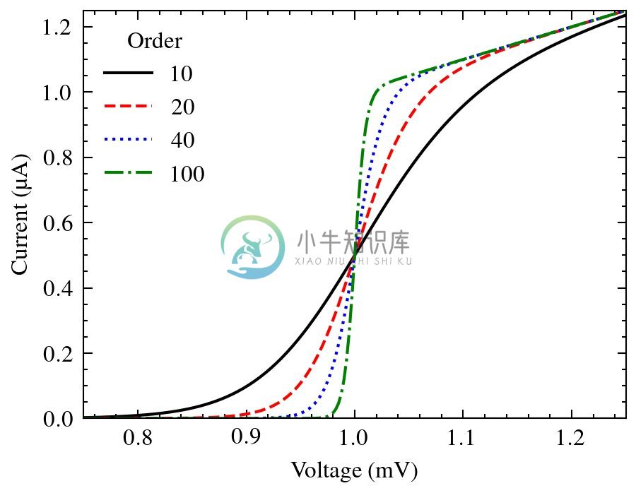
The science + ieee styles for IEEE papers:
- IEEE requires figures to be readable when printed in black and white. The
ieeestyle also sets the figure width to fit within one column of an IEEE paper.
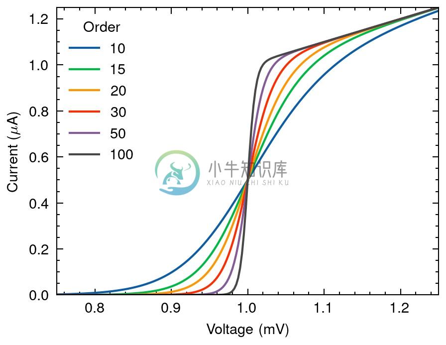
The science + nature styles for Nature articles:
- Nature recommends sans-serif fonts.
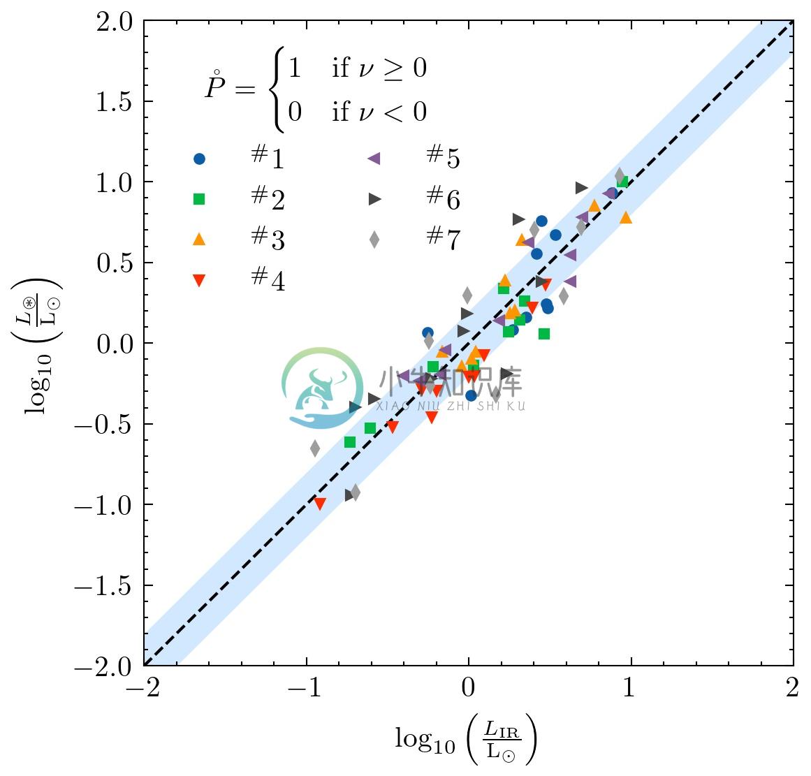
The science + scatter styles for scatter plots:
The science + notebook styles for Jupyter notebooks:
You can also combine these styles with the other styles that come with Matplotlib. For example, the dark_background + science + high-vis styles:
Note: See the examples/ directory for more!
CJK Fonts
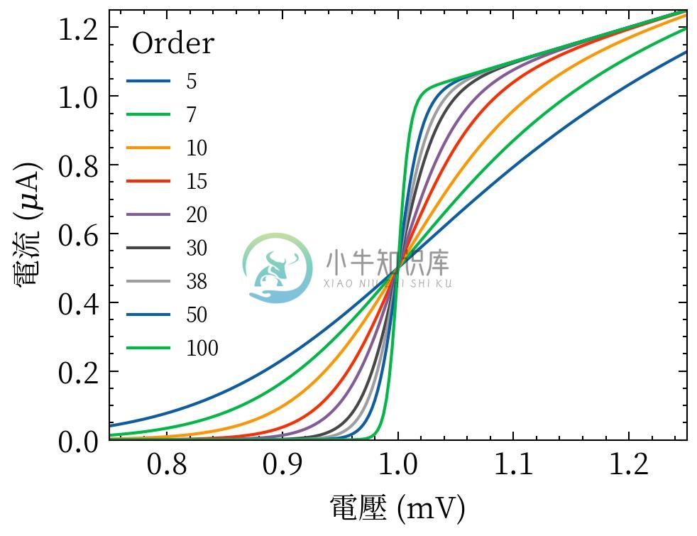
Traditional Chinese (science + no-latex + cjk-tc-font):
Simplified Chinese (science + no-latex + cjk-sc-font):
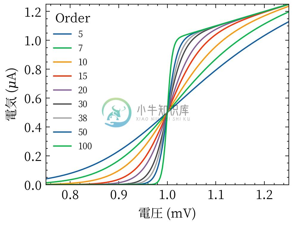
Japanese (science + no-latex + cjk-jp-font):
Korean (science + no-latex + cjk-kr-font):
See the FAQ for information on installing CJK fonts.
Other Languages
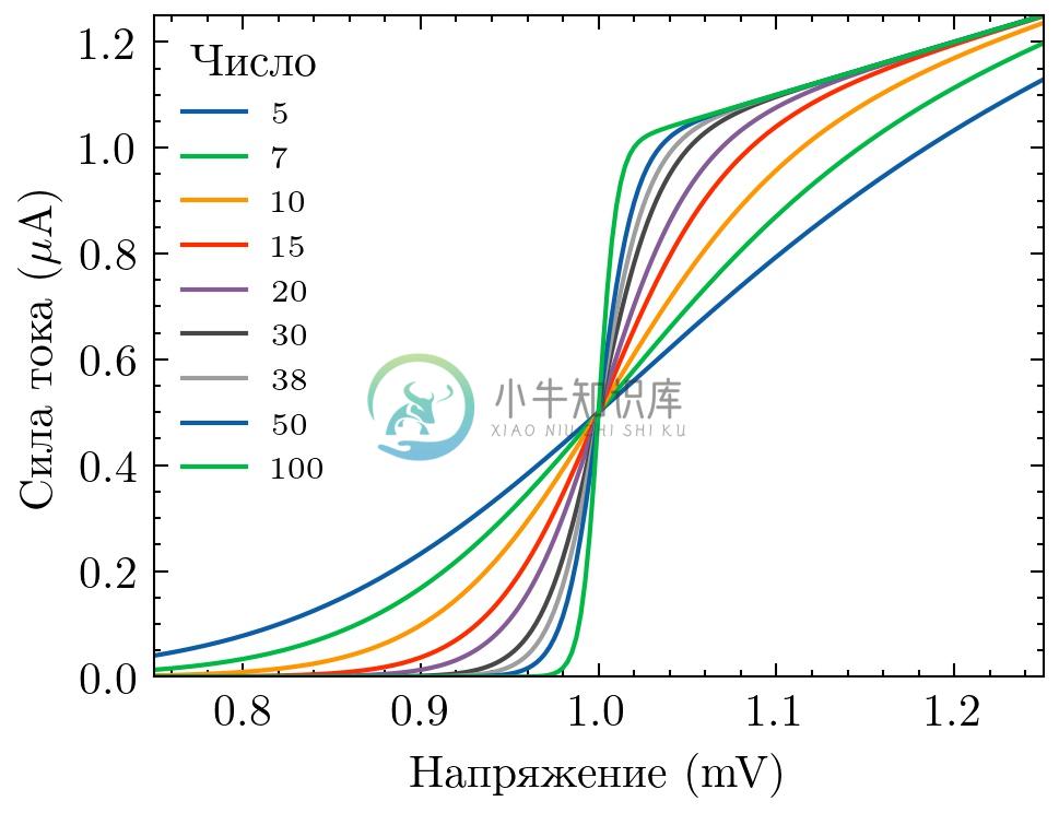
Russian/cyrillic (science + russian-font):
Color Blind Safe Color Cycles
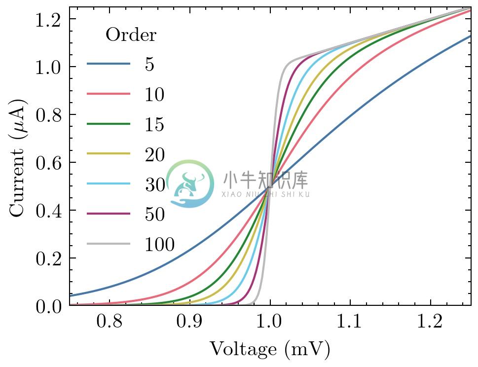
The bright color cycle (7 colors):
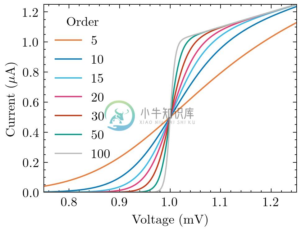
The vibrant color cycle (7 colors):
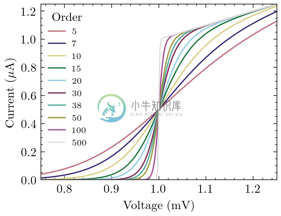
The muted color cycle (10 colors):
The high-contrast color cycle (3 colors):
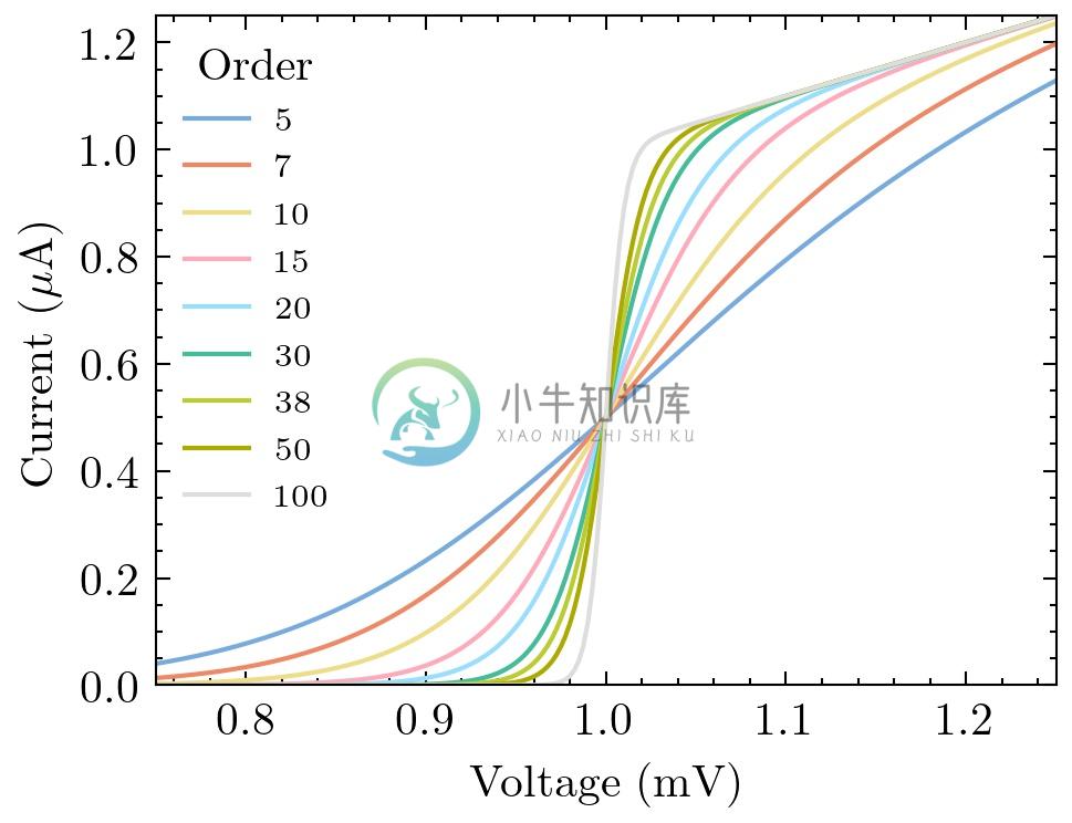
The light color cycle (9 colors):
Note: These color cycles are from Paul Tol's website.
Other Color Cycles
The std-colors color cycle (used to override other color cycles, e.g., the color cycle from ieee):
The high-vis color cycle:
The retro color cycle:
Help and Contributing
Please feel free to contribute to the SciencePlots repo! For example, it would be good to add new styles for different journals and add new color cycles. Before starting a new style or making any changes, please create an issue through the GitHub issue tracker. That way we can discuss if the changes are necessary and the best approach.
If you need any help with SciencePlots, please first check the FAQ and search through the previous GitHub issues. If you can't find an answer, create a new issue through the GitHub issue tracker.
You can checkout Matplotlib's documentation for more information on plotting settings.
FAQ
Installing Latex:
SciencePlots requires Latex to be installed on your machine.
On MacOS, I recommend MacTex. Make sure that this Latex installation is added to your path enviroment variable. See this issue for more troubleshooting tips.
On Windows, I recommend MikTex. Again, you have to add Latex to your path enviroment variable. See this issue for more troubleshooting tips.
On Linux (Ubuntu), you can install Tex Live and the other requirements using:
sudo apt-get install dvipng texlive-latex-extra texlive-fonts-recommended cm-super
Please see Matplotlib's guide to using Latex for more troubleshooting tips.
If you don't want to install Latex, you can disable Latex by using:
plt.style.use(['science','no-latex'])
Installing CJK fonts
To use Chinese, Japanese or Korean fonts, you first need to install Noto CJK Fonts. You can download and install these fonts from the given link or you can install them with a package manager:
# Ubuntu / Debian
sudo apt update
sudo apt install fonts-noto-cjk

# macOS
brew tap homebrew/cask-fonts
brew cask install font-noto-serif-cjk-tc
brew cask install font-noto-serif-cjk-sc
brew cask install font-noto-serif-cjk-jp
brew cask install font-noto-serif-cjk-kr

# archlinux
sudo pacman -S noto-fonts-cjk
For Windows Subsystem for Linux (WSL), you will need to manually download and install the fonts by following these instructions.
Note that
matplotlibmay not find the fonts correctly. You can refresh the font cache by running:import matplotlib.font_manager as fm fm._rebuild()
See this issue for more information.
Installing SciencePlots manually:
If you like, you can install the
*.mplstylefiles manually. First, clone the repository and then copy all of the*.mplstylefiles into your Matplotlib style directory. If you're not sure where this is, in an interactive python console type:import matplotlib print(matplotlib.get_configdir())
You should get back something like
/home/garrett/.matplotlib. You would then put the*.mplstylefiles in/home/garrett/.matplotlib/stylelib/(you may need to create thestylelibdirectory):cp styles/*/*.mplstyle ~/.matplotlib/stylelib/
Using different fonts:
SciencePlots uses the default serif font. If you would like to specify a different font, you can use:
import matplotlib.pyplot as plt
plt.style.use('science')
plt.rcParams.update({
    "font.family": "serif",   # specify font family here
    "font.serif": ["Times"],  # specify font here
    "font.size":11})          # specify font size here
If you would like to use Times New Roman specifically, please see the discussion in this issue.
Installing SciencePlots within Google Colab, IPython, Jupyter Notebooks, etc.:
After installing SciencePlots within one of these environments, you may need to reload the Matplotlib style library. For example:
!pip install SciencePlots
import matplotlib.pyplot as plt
plt.style.reload_library()
plt.style.use('science')
SciencePlots in Academic Papers
The following papers use SciencePlots:
Y. Liu, X. Liu, Y. Sun, "QGrain: An open-source and easy-to-use software for the comprehensive analysis of grain size distributions", Sedimentary Geology, vol. 423, 105980, Aug. 2021.
J. Garrett, and E. Tong, "A Dispersion-Compensated Algorithm for the Analysis of Electromagnetic Waveguides," IEEE Signal Process. Lett., vol. 28, pp. 1175-1179, Jun. 2021.
G. Jegannathan, et al., "Current-Assisted SPAD with Improved p-n Junction and Enhanced NIR Performance", Sensors, Dec 2020. (open access)
H. Tian, et al., "ivis Dimensionality Reduction Framework for Biomacromolecular Simulations", J. Chem. Inf. Model., Aug 2020. (open access)
P. Stoltz, et al., "A new simple algorithm for space charge limited emission," Phys. Plasmas, vol. 27, no. 9, pp. 093103, Sep. 2020. (open access)
J. Garrett, et al., "A Nonlinear Transmission Line Model for Simulating Distributed SIS Frequency Multipliers," IEEE Trans. THz Sci. Technol., vol. 10, no. 3, pp. 246-255, May 2020. (open access)
J. Garrett, et al., "Simulating the Behavior of a 230 GHz SIS Mixer Using Multi-Tone Spectral Domain Analysis," IEEE Trans. THz Sci. Technol., vol. 9, no. 9, pp. 540-548, Nov. 2019. (open access)
J. Garrett, et al., "A Compact and Easy to Fabricate E-plane Waveguide Bend," IEEE Microw. Wireless Compon. Lett., vol. 29, no. 8, pp. 529-531, Aug. 2019. (open access)
J. Garrett, "A 230 GHz Focal Plane Array Using a Wide IF Bandwidth SIS Receiver," DPhil thesis, University of Oxford, Oxford, UK, 2018. (open access)
If you use SciencePlots in your paper/thesis, feel free to add it to the list!
Citing SciencePlots
You don't have to cite SciencePlots if you use it but it's nice if you do:
@article{SciencePlots,
  author       = {John D. Garrett},
  title        = {{garrettj403/SciencePlots}},
  month        = sep,
  year         = 2021,
  publisher    = {Zenodo},
  version      = {1.0.9},
  doi          = {10.5281/zenodo.4106649},
  url          = {http://doi.org/10.5281/zenodo.4106649}
}
-
SciencePlots SciencePlots简介: 一款论文绘图的工具包_NsfNSF的博客-CSDN博客 Python Matplotlib 与 Latex的联用(附带TeXLive安装过程)_GovenSun的博客-CSDN博客_python texlive


