Oceananigans.jl

�� Fast and friendly ocean-flavored Julia software for simulating incompressible fluid dynamics in Cartesian and spherical shell domains on CPUs and GPUs. https://clima.github.io/OceananigansDocumentation/stable

Oceananigans.jl is a fast and friendly fluid flow solver written in Julia that can be run in 1-3 dimensions on CPUs and GPUs. It can simulate the incompressible Boussinesq equations, the shallow water equations, or the hydrostatic Boussinesq equations with a free surface. Oceananigans.jl comes with user-friendly features for simulating rotating stratified fluids including user-defined boundary conditions and forcing functions, arbitrary tracers, large eddy simulation turbulence closures, high-order advection schemes, immersed boundaries, Lagrangian particle tracking, and more!

We strive for a user interface that makes Oceananigans.jl as friendly and intuitive to use as possible, allowing users to focus on the science. Internally, we have attempted to write the underlying algorithm so that the code runs as fast as possible for the configuration chosen by the user --- from simple two-dimensional setups to complex three-dimensional simulations --- and so that as much code as possible is shared between the different architectures, models, and grids.

Contents

• Installation instructions
• Running your first model
• Getting help
• Contributing
• Movies
• Performance benchmarks

Installation instructions

You can install the latest version of Oceananigans using the built-in package manager (accessed by pressing ] in the Julia command prompt) to add the package and instantiate/build all depdendencies

julia>]
(v1.6) pkg> add Oceananigans
(v1.6) pkg> instantiate

We recommend installing Oceananigans with the built-in Julia package manager, because this installs a stable, tagged release. Oceananigans.jl can be updated to the latest tagged release from the package manager by typing

(v1.6) pkg> update Oceananigans

At this time, updating should be done with care, as Oceananigans is under rapid development and breaking changes to the user API occur often. But if anything does happen, please open an issue!

Note: The latest version of Oceananigans requires at least Julia v1.6 to run. Installing Oceananigans with an older version of Julia will install an older version of Oceananigans (the latest version compatible with your version of Julia).

Running your first model

Let's initialize a 3D horizontally periodic model with 100×100×50 grid points on a 2×2×1 km domain and simulate it for 1 hour using a constant time step of 60 seconds.

using Oceananigans
grid = RegularRectilinearGrid(size=(100, 100, 50), extent=(2π, 2π, 1))
model = NonhydrostaticModel(grid=grid)
simulation = Simulation(model, Δt=60, stop_time=3600)
run!(simulation)

You just simulated what might have been a 3D patch of ocean, it's that easy! It was a still lifeless ocean so nothing interesting happened but now you can add interesting dynamics and visualize the output.

More interesting example

Let's add something to make the dynamics a bit more interesting. We can add a hot bubble in the middle of the domain and watch it rise to the surface. This example also shows how to set an initial condition.

using Oceananigans

N = Nx = Ny = Nz = 128   # Number of grid points in each dimension.
L = Lx = Ly = Lz = 2000  # Length of each dimension.
topology = (Periodic, Periodic, Bounded)

model = NonhydrostaticModel(
    architecture = CPU(),
            grid = RegularRectilinearGrid(topology=topology, size=(Nx, Ny, Nz), extent=(Lx, Ly, Lz)),
         closure = IsotropicDiffusivity(ν=4e-2, κ=4e-2)
)

# Set a temperature perturbation with a Gaussian profile located at the center.
# This will create a buoyant thermal bubble that will rise with time.
x₀, z₀ = Lx/2, Lz/2
T₀(x, y, z) = 20 + 0.01 * exp(-100 * ((x - x₀)^2 + (z - z₀)^2) / (Lx^2 + Lz^2))
set!(model, T=T₀)

simulation = Simulation(model, Δt=10, stop_iteration=5000)
run!(simulation)

By changing architecture = CPU() to architecture = GPU() the example will run on a CUDA-enabled Nvidia GPU!

You can see some movies from GPU simulations below along with CPU and GPU performance benchmarks.

Getting help

If you are interested in using Oceananigans.jl or are trying to figure out how to use it, please feel free to ask us questions and get in touch! If you're trying to set up a model then check out the examples and model setup documentation. Check out the examples and please feel free to start a discussion if you have any questions, comments, suggestions, etc! There is also an #oceananigans channel on the Julia Slack.

Citing

If you use Oceananigans.jl as part of your research, teaching, or other activities, we would be grateful if you could cite our work and mention Oceananigans.jl by name.

@article{OceananigansJOSS,
  doi = {10.21105/joss.02018},
  url = {https://doi.org/10.21105/joss.02018},
  year = {2020},
  publisher = {The Open Journal},
  volume = {5},
  number = {53},
  pages = {2018},
  author = {Ali Ramadhan and Gregory LeClaire Wagner and Chris Hill and Jean-Michel Campin and Valentin Churavy and Tim Besard and Andre Souza and Alan Edelman and Raffaele Ferrari and John Marshall},
  title = {Oceananigans.jl: Fast and friendly geophysical fluid dynamics on GPUs},
  journal = {Journal of Open Source Software}
}

We also maintain a list of publication using Oceananigans.jl. If you have work using Oceananigans.jl that you would like to have listed there, please open a pull request to add it or let us know!

Contributing

If you're interested in contributing to the development of Oceananigans we want your help no matter how big or small a contribution you make! It's always great to have new people look at the code with fresh eyes: you will see errors that other developers have missed.

Let us know by opening an issue if you'd like to work on a new feature or if you're new to open-source and want to find a cool little project or issue to work on that fits your interests! We're more than happy to help along the way.

For more information, check out our contributor's guide.

Movies

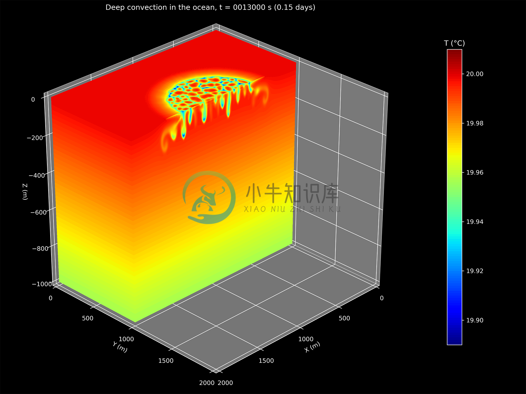
Deep convection

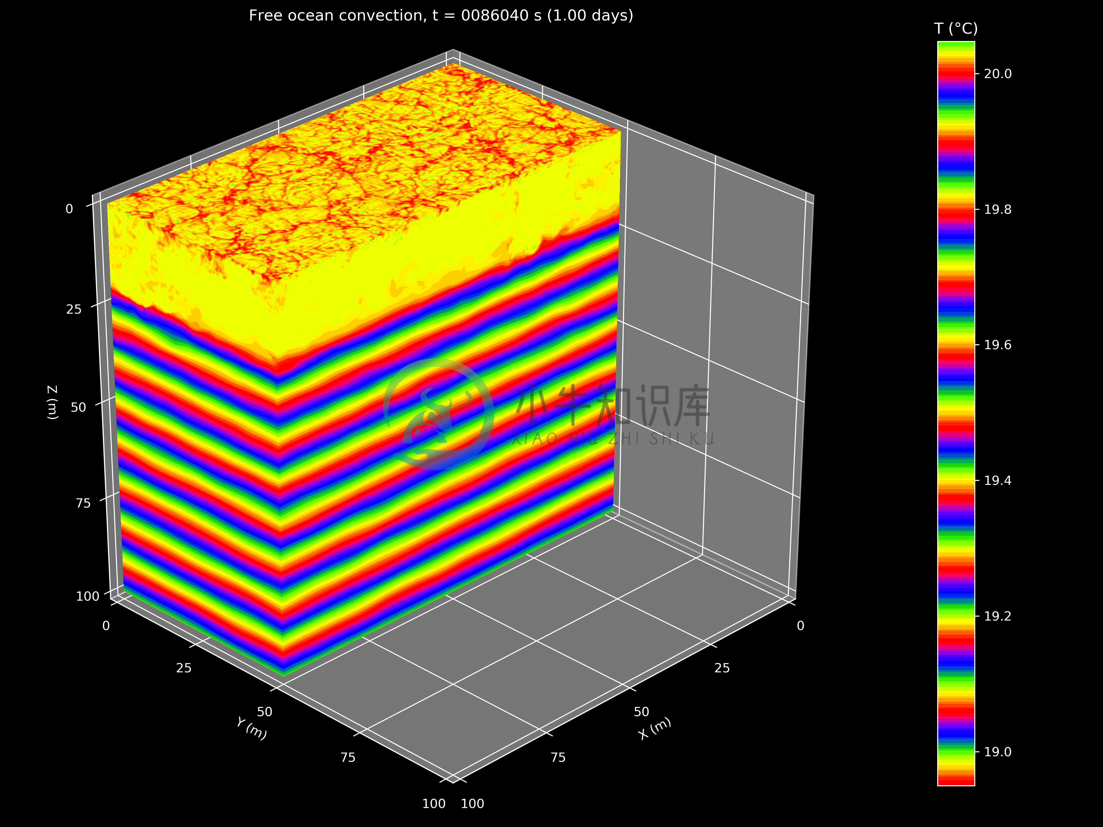
Free convection

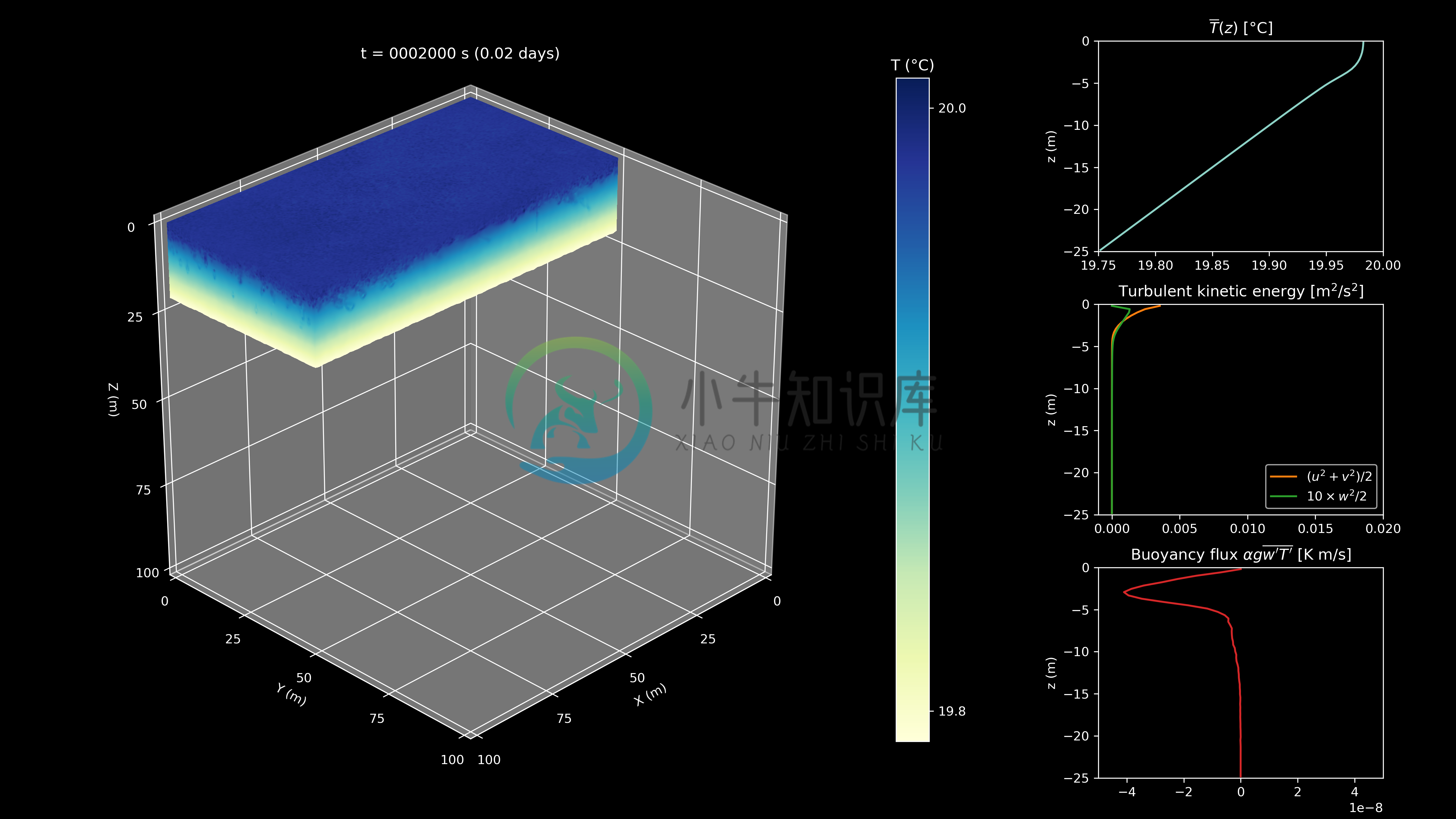
Winds blowing over the ocean

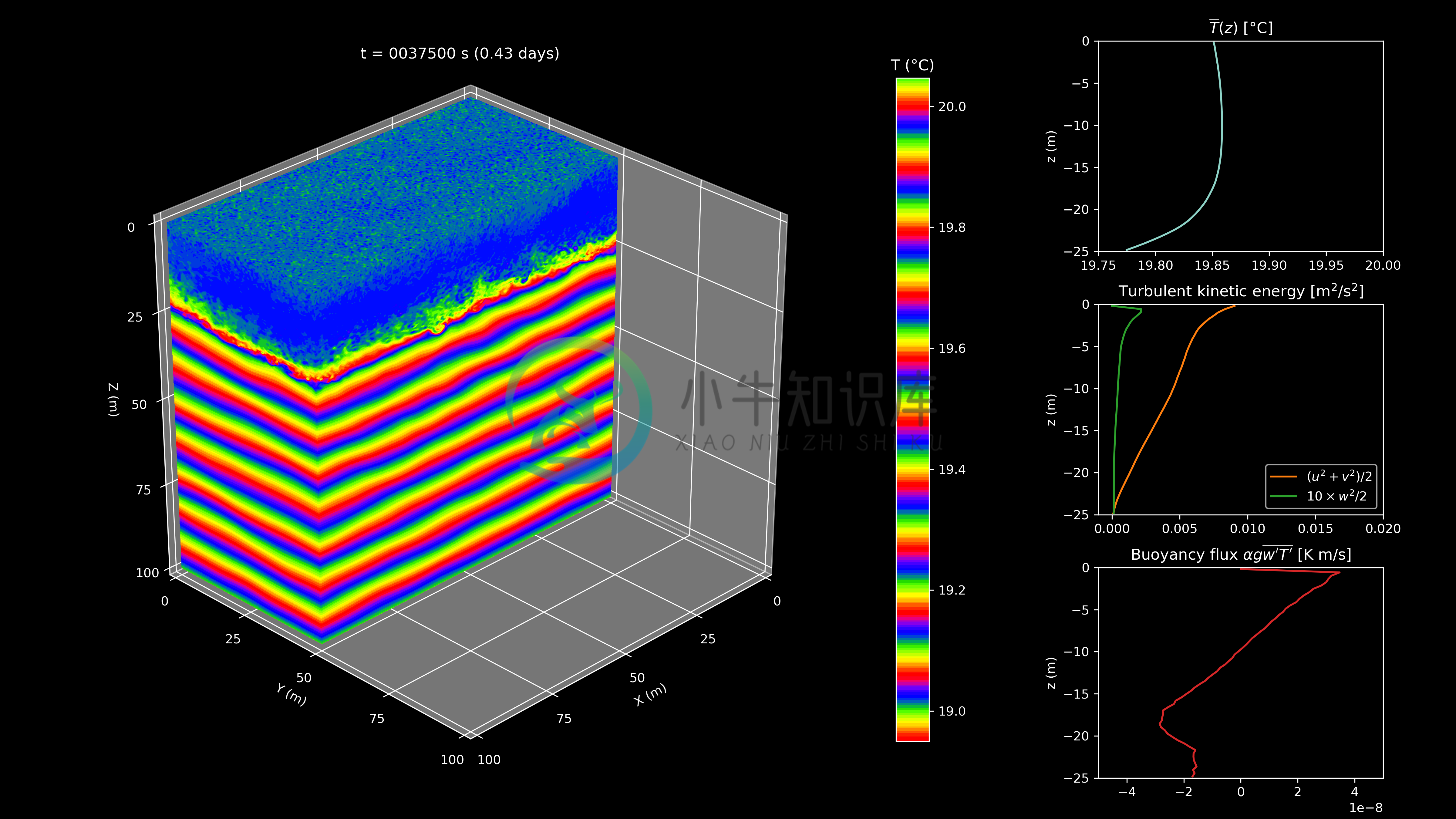
Free convection with wind stress

Performance benchmarks

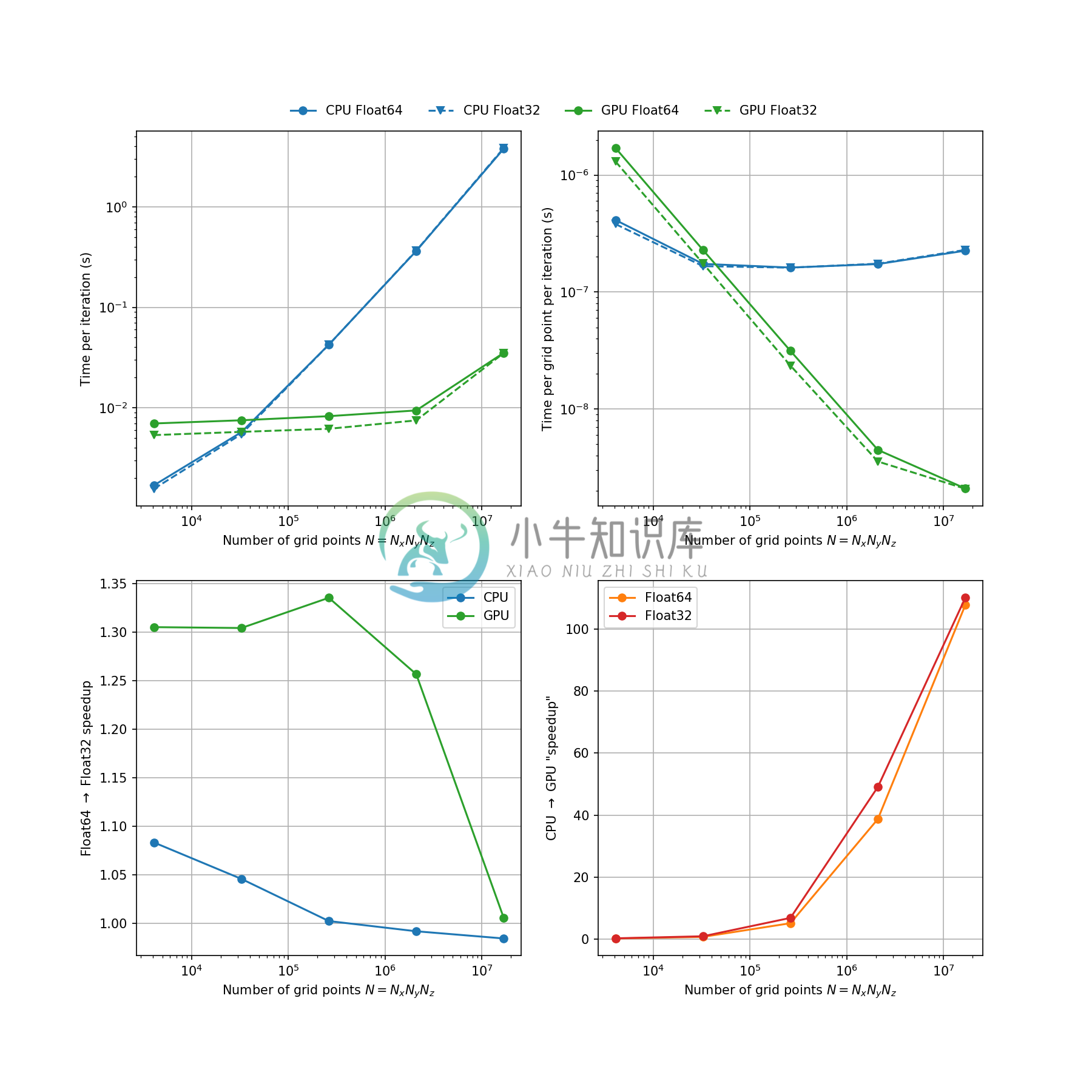
We've performed some preliminary performance benchmarks (see the performance benchmarks section of the documentation) by initializing models of various sizes and measuring the wall clock time taken per model iteration (or time step).

This is not really a fair comparison as we haven't parallelized across all the CPU's cores so we will revisit these benchmarks once Oceananigans.jl can run on multiple CPUs and GPUs.

To make full use of or fully saturate the computing power of a GPU such as an Nvidia Tesla V100 ora Titan V, the model should have around ~10 million grid points or more.

Sometimes counter-intuitively running with Float32 is slower than Float64. This is likely dueto type mismatches causing slowdowns as floats have to be converted between 32-bit and 64-bit, anissue that needs to be addressed meticulously. Due to other bottlenecks such as memory accesses andGPU register pressure, Float32 models may not provide much of a speedup so the main benefit becomeslower memory costs (by around a factor of 2).